Perovskite light-intensity dependant JV fits with SIMsalabim (real data)
This notebook is a demonstration of how to fit light-intensity dependent JV curves with drift-diffusion models using the SIMsalabim package.
[1]:
# Import necessary libraries
import warnings, os, sys, shutil
# remove warnings from the output
os.environ["PYTHONWARNINGS"] = "ignore"
warnings.filterwarnings(action='ignore', category=FutureWarning)
warnings.filterwarnings(action='ignore', category=UserWarning)
import pandas as pd
import matplotlib.pyplot as plt
import numpy as np
from numpy.random import default_rng
from scipy import constants
import torch, copy, uuid
import pySIMsalabim as sim
from pySIMsalabim.experiments.JV_steady_state import *
import ax, logging
from ax.utils.notebook.plotting import init_notebook_plotting, render
init_notebook_plotting() # for Jupyter notebooks
try:
from optimpv import *
from optimpv.optimizers.axBOtorch.axUtils import *
except Exception as e:
sys.path.append('../') # add the path to the optimpv module
from optimpv import *
from optimpv.optimizers.axBOtorch.axUtils import *
[INFO 01-20 11:02:54] ax.utils.notebook.plotting: Injecting Plotly library into cell. Do not overwrite or delete cell.
[INFO 01-20 11:02:54] ax.utils.notebook.plotting: Please see
(https://ax.dev/tutorials/visualizations.html#Fix-for-plots-that-are-not-rendering)
if visualizations are not rendering.
Get the experimental data
[2]:
# Set the session path for the simulation and the input files
session_path = os.path.join(os.path.join(os.path.abspath('../'),'SIMsalabim','SimSS'))
input_path = os.path.join(os.path.join(os.path.join(os.path.abspath('../'),'Data','simsalabim_test_inputs','JVrealPerovskite')))
simulation_setup_filename = 'simulation_setup_realPerovskite.txt'
simulation_setup = os.path.join(session_path, simulation_setup_filename)
optical_files = ['nk_glass.txt','nk_ITO.txt','nk_PTAA.txt','nk_FACsPbIBr.txt','nk_C60_1.txt','nk_Au.txt']
# path to the layer files defined in the simulation_setup file
l1 = 'PTAA.txt'
l2 = 'perovskite.txt'
l3 = 'C60.txt'
l1 = os.path.join(input_path, l1)
l2 = os.path.join(input_path, l2)
l3 = os.path.join(input_path, l3)
# copy this files to session_path
force_copy = True
if not os.path.exists(session_path):
os.makedirs(session_path)
for file in [l1,l2,l3,simulation_setup_filename]:
file = os.path.join(input_path, os.path.basename(file))
if force_copy or not os.path.exists(os.path.join(session_path, os.path.basename(file))):
shutil.copyfile(file, os.path.join(session_path, os.path.basename(file)))
else:
print('File already exists: ',file)
# copy the optical files to the session path
for file in optical_files:
file = os.path.join(input_path, os.path.basename(file))
if force_copy or not os.path.exists(os.path.join(session_path, os.path.basename(file))):
shutil.copyfile(file, os.path.join(session_path, os.path.basename(file)))
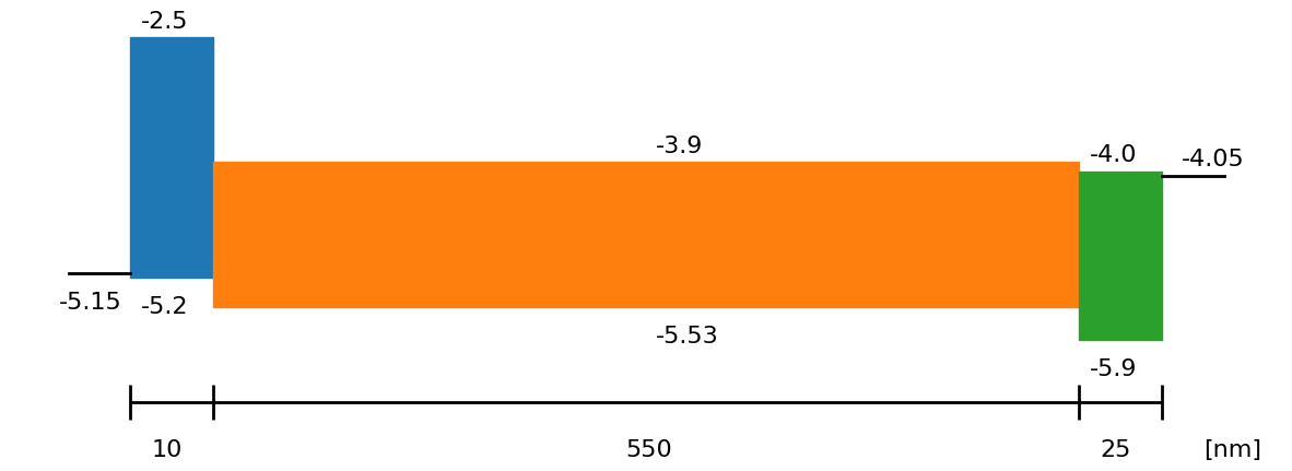
# Show the device structure
fig = sim.plot_band_diagram(simulation_setup, session_path)
dev_par, layers = sim.load_device_parameters(session_path, simulation_setup, run_mode = False)
SIMsalabim_params = {}
for layer in layers:
SIMsalabim_params[layer[1]] = sim.ReadParameterFile(os.path.join(session_path,layer[2]))
L_active_Layer = float(SIMsalabim_params['l2']['L'])
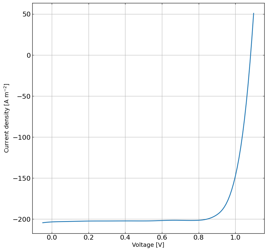
# Load the JV data
df = pd.read_csv(os.path.join(input_path, 'JV_realPerovskite.dat'), sep=' ')
X = df['Vext'].values
y = df['Jext'].values
Gfracs = None
# get 1sun Jsc as it will help narrow down the range for Gehp
Jsc_1sun = np.interp(0.0, X, y)
minJ = np.max(y) # max because we have positive current density in the file
q = constants.value(u'elementary charge')
G_ehp_calc = abs(Jsc_1sun/(q*L_active_Layer))
G_ehp_max = abs(minJ/(q*L_active_Layer))
# plot the data for each Gfrac
plt.figure(figsize=(10,10))
plt.plot(X, y, '-')
plt.grid()
plt.xlabel('Voltage [V]')
plt.ylabel('Current density [A m$^{-2}$]')
plt.show()
Define the parameters for the simulation
[3]:
params = [] # list of parameters to be optimized
mun = FitParam(name = 'l2.mu_n', value = 8e-5, bounds = [1e-5,1e-2], values = None, start_value = None, log_scale = True, value_type = 'float', fscale = None, rescale = False, stepsize = None, display_name=r'$\mu_n$', unit='m$^2$ V$^{-1}$s$^{-1}$', axis_type = 'log', std = 0,encoding = None,force_log = False)
params.append(mun)
mup = FitParam(name = 'l2.mu_p', value = 8e-5, bounds = [1e-5,1e-2], values = None, start_value = None, log_scale = True, value_type = 'float', fscale = None, rescale = False, stepsize = None, display_name=r'$\mu_p$', unit='m$^2$ V$^{-1}$s$^{-1}$', axis_type = 'log', std = 0,encoding = None,force_log = False)
params.append(mup)
bulk_tr = FitParam(name = 'l2.N_t_bulk', value = 5.1e20, bounds = [1e19,1e22], values = None, start_value = None, log_scale = True, value_type = 'float', fscale = None, rescale = False, stepsize = None, display_name=r'$N_{T}$', unit='s', axis_type = 'log', std = 0,encoding = None,force_log = False)
params.append(bulk_tr)
Nions = FitParam(name = 'l2.N_ions', value = 4e22, bounds = [1e22,5e22], type='range', values = None, start_value = None, log_scale = True, value_type = 'float', fscale = None, rescale = False, stepsize = None, display_name=r'$N_{ions}$', unit='m$^{-3}$', axis_type = 'log', std = 0,encoding = None,force_log = False)
params.append(Nions)
N_t_int_l1 = FitParam(name = 'l1.N_t_int', value = 5e12, bounds = [5e11,5e13], values = None, start_value = None, log_scale = True, value_type = 'float', fscale = None, rescale = False, stepsize = None, display_name=r'$N_{T,int}^{HTL}$', unit='m$^{-2}$', axis_type = 'log', std = 0,encoding = None,force_log = False)
params.append(N_t_int_l1)
N_t_int_l2 = FitParam(name = 'l2.N_t_int', value = 4e12, bounds = [5e11,5e13], values = None, start_value = None, log_scale = True, value_type = 'float', fscale = None, rescale = False, stepsize = None, display_name=r'$N_{T,int}^{ETL}$', unit='m$^{-2}$', axis_type = 'log', std = 0,encoding = None,force_log = False)
params.append(N_t_int_l2)
R_series = FitParam(name = 'R_series', value = 1e-4, bounds = [1e-6,1e-2], log_scale = True, value_type = 'float', fscale = None, rescale = False, display_name=r'$R_{series}$', unit=r'$\Omega$ m$^2$', axis_type = 'log', force_log = False)
params.append(R_series)
R_shunt = FitParam(name = 'R_shunt', value = 1e1, bounds = [1e-2,1e2], log_scale = True, value_type = 'float', fscale = None, rescale = False, display_name=r'$R_{shunt}$', unit=r'$\Omega$ m$^2$', axis_type = 'log', force_log = False)
params.append(R_shunt)
# save the original parameters for later
params_orig = copy.deepcopy(params)
num_free_params = len([p for p in params if p.type != 'fixed'])
Run the optimization
[4]:
# Define the Agent and the target metric/loss function
from optimpv.models.DDfits.JVAgent import JVAgent
metric = 'nrmse' # can be 'nrmse', 'mse', 'mae'
loss = 'linear' # can be 'linear', 'huber', 'soft_l1'
jv = JVAgent(params, X, y, session_path, simulation_setup, parallel = False, max_jobs = 1, metric = metric, loss = loss)
[5]:
from optimpv.optimizers.axBOtorch.axBOtorchOptimizer import axBOtorchOptimizer
from optimpv.optimizers.axBOtorch.axUtils import get_VMLC_default_model_kwargs_list
# Define the optimizer
optimizer = axBOtorchOptimizer(params = params, agents = jv, models = ['SOBOL','BOTORCH_MODULAR'],n_batches = [1,45], batch_size = [10,2], model_kwargs_list = get_VMLC_default_model_kwargs_list(num_free_params))
[6]:
# optimizer.optimize() # run the optimization with ax
optimizer.optimize_turbo() # run the optimization with turbo
[INFO 01-20 11:02:54] optimpv.axBOtorchOptimizer: Starting optimization with 46 batches and a total of 100 trials
[INFO 01-20 11:02:54] optimpv.axBOtorchOptimizer: Starting Sobol batch 1 with 10 trials
[INFO 01-20 11:02:57] optimpv.axBOtorchOptimizer: Finished Sobol with best value of 0.123471
[INFO 01-20 11:03:00] optimpv.axBOtorchOptimizer: Finished Turbo batch 2 with 2 trials with current best value: 2.5202e-02, TR length: 8.00e-01
[INFO 01-20 11:03:01] optimpv.axBOtorchOptimizer: Finished Turbo batch 3 with 2 trials with current best value: 2.5202e-02, TR length: 8.00e-01
[INFO 01-20 11:03:03] optimpv.axBOtorchOptimizer: Finished Turbo batch 4 with 2 trials with current best value: 2.5202e-02, TR length: 8.00e-01
[INFO 01-20 11:03:05] optimpv.axBOtorchOptimizer: Finished Turbo batch 5 with 2 trials with current best value: 2.5202e-02, TR length: 8.00e-01
[INFO 01-20 11:03:06] optimpv.axBOtorchOptimizer: Finished Turbo batch 6 with 2 trials with current best value: 1.3314e-02, TR length: 8.00e-01
[INFO 01-20 11:03:08] optimpv.axBOtorchOptimizer: Finished Turbo batch 7 with 2 trials with current best value: 1.3314e-02, TR length: 8.00e-01
[INFO 01-20 11:03:09] optimpv.axBOtorchOptimizer: Finished Turbo batch 8 with 2 trials with current best value: 1.2716e-02, TR length: 8.00e-01
[INFO 01-20 11:03:11] optimpv.axBOtorchOptimizer: Finished Turbo batch 9 with 2 trials with current best value: 1.2716e-02, TR length: 8.00e-01
[INFO 01-20 11:03:12] optimpv.axBOtorchOptimizer: Finished Turbo batch 10 with 2 trials with current best value: 1.2716e-02, TR length: 8.00e-01
[INFO 01-20 11:03:14] optimpv.axBOtorchOptimizer: Finished Turbo batch 11 with 2 trials with current best value: 1.2716e-02, TR length: 8.00e-01
[INFO 01-20 11:03:15] optimpv.axBOtorchOptimizer: Finished Turbo batch 12 with 2 trials with current best value: 1.2716e-02, TR length: 5.00e-01
[INFO 01-20 11:03:17] optimpv.axBOtorchOptimizer: Finished Turbo batch 13 with 2 trials with current best value: 1.2716e-02, TR length: 5.00e-01
[INFO 01-20 11:03:18] optimpv.axBOtorchOptimizer: Finished Turbo batch 14 with 2 trials with current best value: 1.2716e-02, TR length: 5.00e-01
[INFO 01-20 11:03:20] optimpv.axBOtorchOptimizer: Finished Turbo batch 15 with 2 trials with current best value: 1.1238e-02, TR length: 5.00e-01
[INFO 01-20 11:03:22] optimpv.axBOtorchOptimizer: Finished Turbo batch 16 with 2 trials with current best value: 7.9445e-03, TR length: 5.00e-01
[INFO 01-20 11:03:23] optimpv.axBOtorchOptimizer: Finished Turbo batch 17 with 2 trials with current best value: 7.9445e-03, TR length: 5.00e-01
[INFO 01-20 11:03:25] optimpv.axBOtorchOptimizer: Finished Turbo batch 18 with 2 trials with current best value: 6.1293e-03, TR length: 5.00e-01
[INFO 01-20 11:03:26] optimpv.axBOtorchOptimizer: Finished Turbo batch 19 with 2 trials with current best value: 6.1293e-03, TR length: 5.00e-01
[INFO 01-20 11:03:28] optimpv.axBOtorchOptimizer: Finished Turbo batch 20 with 2 trials with current best value: 6.1293e-03, TR length: 5.00e-01
[INFO 01-20 11:03:29] optimpv.axBOtorchOptimizer: Finished Turbo batch 21 with 2 trials with current best value: 6.1293e-03, TR length: 5.00e-01
[INFO 01-20 11:03:31] optimpv.axBOtorchOptimizer: Finished Turbo batch 22 with 2 trials with current best value: 6.1293e-03, TR length: 3.12e-01
[INFO 01-20 11:03:33] optimpv.axBOtorchOptimizer: Finished Turbo batch 23 with 2 trials with current best value: 6.1293e-03, TR length: 3.12e-01
[INFO 01-20 11:03:34] optimpv.axBOtorchOptimizer: Finished Turbo batch 24 with 2 trials with current best value: 6.1293e-03, TR length: 3.12e-01
[INFO 01-20 11:03:36] optimpv.axBOtorchOptimizer: Finished Turbo batch 25 with 2 trials with current best value: 6.1293e-03, TR length: 3.12e-01
[INFO 01-20 11:03:37] optimpv.axBOtorchOptimizer: Finished Turbo batch 26 with 2 trials with current best value: 6.1293e-03, TR length: 1.95e-01
[INFO 01-20 11:03:39] optimpv.axBOtorchOptimizer: Finished Turbo batch 27 with 2 trials with current best value: 5.5735e-03, TR length: 1.95e-01
[INFO 01-20 11:03:40] optimpv.axBOtorchOptimizer: Finished Turbo batch 28 with 2 trials with current best value: 5.5735e-03, TR length: 1.95e-01
[INFO 01-20 11:03:42] optimpv.axBOtorchOptimizer: Finished Turbo batch 29 with 2 trials with current best value: 5.5735e-03, TR length: 1.95e-01
[INFO 01-20 11:03:43] optimpv.axBOtorchOptimizer: Finished Turbo batch 30 with 2 trials with current best value: 5.5735e-03, TR length: 1.95e-01
[INFO 01-20 11:03:45] optimpv.axBOtorchOptimizer: Finished Turbo batch 31 with 2 trials with current best value: 5.5735e-03, TR length: 1.22e-01
[INFO 01-20 11:03:47] optimpv.axBOtorchOptimizer: Finished Turbo batch 32 with 2 trials with current best value: 5.5735e-03, TR length: 1.22e-01
[INFO 01-20 11:03:48] optimpv.axBOtorchOptimizer: Finished Turbo batch 33 with 2 trials with current best value: 5.5735e-03, TR length: 1.22e-01
[INFO 01-20 11:03:50] optimpv.axBOtorchOptimizer: Finished Turbo batch 34 with 2 trials with current best value: 5.5735e-03, TR length: 1.22e-01
[INFO 01-20 11:03:51] optimpv.axBOtorchOptimizer: Finished Turbo batch 35 with 2 trials with current best value: 5.5735e-03, TR length: 7.63e-02
[INFO 01-20 11:03:53] optimpv.axBOtorchOptimizer: Finished Turbo batch 36 with 2 trials with current best value: 5.5735e-03, TR length: 7.63e-02
[INFO 01-20 11:03:54] optimpv.axBOtorchOptimizer: Finished Turbo batch 37 with 2 trials with current best value: 5.5735e-03, TR length: 7.63e-02
[INFO 01-20 11:03:56] optimpv.axBOtorchOptimizer: Finished Turbo batch 38 with 2 trials with current best value: 5.5735e-03, TR length: 7.63e-02
[INFO 01-20 11:03:57] optimpv.axBOtorchOptimizer: Finished Turbo batch 39 with 2 trials with current best value: 5.5735e-03, TR length: 4.77e-02
[INFO 01-20 11:03:59] optimpv.axBOtorchOptimizer: Finished Turbo batch 40 with 2 trials with current best value: 5.5548e-03, TR length: 4.77e-02
[INFO 01-20 11:04:01] optimpv.axBOtorchOptimizer: Finished Turbo batch 41 with 2 trials with current best value: 5.5548e-03, TR length: 4.77e-02
[INFO 01-20 11:04:02] optimpv.axBOtorchOptimizer: Finished Turbo batch 42 with 2 trials with current best value: 5.4680e-03, TR length: 4.77e-02
[INFO 01-20 11:04:04] optimpv.axBOtorchOptimizer: Finished Turbo batch 43 with 2 trials with current best value: 5.4680e-03, TR length: 4.77e-02
[INFO 01-20 11:04:05] optimpv.axBOtorchOptimizer: Finished Turbo batch 44 with 2 trials with current best value: 5.4680e-03, TR length: 4.77e-02
[INFO 01-20 11:04:07] optimpv.axBOtorchOptimizer: Finished Turbo batch 45 with 2 trials with current best value: 5.4490e-03, TR length: 4.77e-02
[INFO 01-20 11:04:09] optimpv.axBOtorchOptimizer: Finished Turbo batch 46 with 2 trials with current best value: 5.4490e-03, TR length: 4.77e-02
[INFO 01-20 11:04:10] optimpv.axBOtorchOptimizer: Finished Turbo batch 47 with 2 trials with current best value: 5.4490e-03, TR length: 4.77e-02
[INFO 01-20 11:04:11] optimpv.axBOtorchOptimizer: Turbo is terminated.
[7]:
# get the best parameters and update the params list in the optimizer and the agent
ax_client = optimizer.ax_client # get the ax client
optimizer.update_params_with_best_balance() # update the params list in the optimizer with the best parameters
jv.params = optimizer.params # update the params list in the agent with the best parameters
# print the best parameters
print('Best parameters:')
for p in optimizer.params:
print(p.name, 'fitted value:', p.value)
print('\nSimSS command line:')
print(jv.get_SIMsalabim_clean_cmd(jv.params)) # print the simss command line with the best parameters
Best parameters:
l2.mu_n fitted value: 0.006915539807657599
l2.mu_p fitted value: 0.006993370577441108
l2.N_t_bulk fitted value: 5.092620365209398e+21
l2.N_ions fitted value: 4.980150550037934e+22
l1.N_t_int fitted value: 16406772029238.389
l2.N_t_int fitted value: 17383124899716.56
R_series fitted value: 0.0002050177909866671
R_shunt fitted value: 14.630390539625763
SimSS command line:
./simss -l2.mu_n 0.006915539807657599 -l2.mu_p 0.006993370577441108 -l2.N_t_bulk 5.092620365209398e+21 -l2.N_anion 4.980150550037934e+22 -l2.N_cation 4.980150550037934e+22 -l1.N_t_int 16406772029238.389 -l2.N_t_int 17383124899716.56 -R_series 0.0002050177909866671 -R_shunt 14.630390539625763
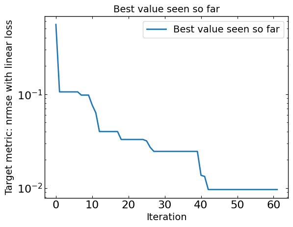
[8]:
# Plot optimization results
data = ax_client.summarize()
all_metrics = optimizer.all_metrics
plt.figure()
plt.plot(np.minimum.accumulate(data[all_metrics]), label="Best value seen so far")
plt.yscale("log")
plt.xlabel("Iteration")
plt.ylabel("Target metric: " + metric + " with " + loss + " loss")
plt.legend()
plt.title("Best value seen so far")
print("Best value seen so far is ", min(data[all_metrics[0]]), "at iteration ", int(data[all_metrics[0]].idxmin()))
plt.show()
Best value seen so far is 0.005448989821527168 at iteration 96
[9]:
from ax.analysis.plotly.parallel_coordinates import ParallelCoordinatesPlot
analysis = ParallelCoordinatesPlot()
analysis.compute(
experiment=ax_client._experiment,
generation_strategy=ax_client._generation_strategy,
# compute can optionally take in an Adapter directly instead of a GenerationStrategy
adapter=None,
)
Parallel Coordinates for JV_JV_nrmse_linear
The parallel coordinates plot displays multi-dimensional data by representing each parameter as a parallel axis. This plot helps in assessing how thoroughly the search space has been explored and in identifying patterns or clusterings associated with high-performing (good) or low-performing (bad) arms. By tracing lines across the axes, one can observe correlations and interactions between parameters, gaining insights into the relationships that contribute to the success or failure of different configurations within the experiment.
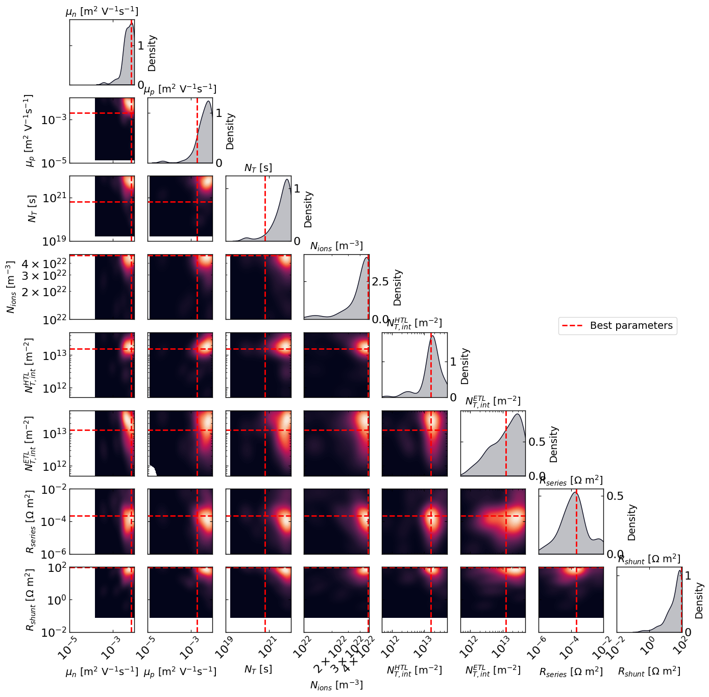
[10]:
# Plot the density of the exploration of the parameters
# this gives a nice visualization of where the optimizer focused its exploration and may show some correlation between the parameters
plot_dens = True
if plot_dens:
from optimpv.posterior.exploration_density import *
best_parameters = {}
for p in optimizer.params:
best_parameters[p.name] = p.value
fig_dens, ax_dens = plot_density_exploration(params, optimizer = optimizer, best_parameters = best_parameters, optimizer_type = 'ax')
[11]:
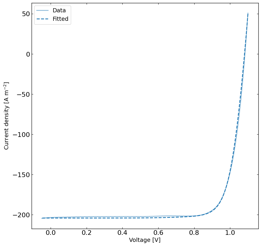
# rerun the simulation with the best parameters
yfit = jv.run(parameters={}) # run the simulation with the best parameters
plt.figure(figsize=(10,10))
linewidth = 2
plt.plot(X, y, 'C0-',label='Data',linewidth=linewidth, alpha=0.5)
plt.plot(X, yfit, 'C0--', label='Fitted',linewidth=linewidth)
plt.xlabel('Voltage [V]')
plt.ylabel('Current density [A m$^{-2}$]')
plt.legend()
plt.show()
[12]:
# Clean up the output files (comment out if you want to keep the output files)
sim.clean_all_output(session_path)
sim.delete_folders('tmp',session_path)
# uncomment the following lines to delete specific files
sim.clean_up_output('PTAA',session_path)
sim.clean_up_output('perovskite',session_path)
sim.clean_up_output('C60',session_path)
sim.clean_up_output('simulation_setup_realPerovskite.txt',session_path)