Fitting degradation JV data with Lazy Posterior analysis
This notebook is a demonstration of how to fit light-intensity dependent JV curves with drift-diffusion models using the SIMsalabim package.
In this example, we create synthetic JV data for a device that degrades over time, and then use Bayesian optimization to fit the data and extract the posterior distributions of the parameters using the Lazy Posterior method.
[1]:
# Import necessary libraries
import warnings, os, sys, shutil, matplotlib, ray
# remove warnings from the output
os.environ["PYTHONWARNINGS"] = "ignore"
warnings.filterwarnings(action='ignore', category=FutureWarning)
warnings.filterwarnings(action='ignore', category=UserWarning)
os.environ['PYTORCH_CUDA_ALLOC_CONF'] = 'expandable_segments:True'
import pandas as pd
import matplotlib.pyplot as plt
import numpy as np
from numpy.random import default_rng
import torch, copy, uuid
import pySIMsalabim as sim
from pySIMsalabim.experiments.JV_steady_state import *
import ax, logging
from ax.utils.notebook.plotting import init_notebook_plotting, render
init_notebook_plotting() # for Jupyter notebooks

try:
    from optimpv import *
    from optimpv.optimizers.axBOtorch.axUtils import *
    from optimpv.models.DDfits.JVAgent import JVAgent
    from optimpv.optimizers.axBOtorch.axBOtorchOptimizer import axBOtorchOptimizer
    from optimpv.optimizers.axBOtorch.axUtils import get_VMLC_default_model_kwargs_list
except Exception as e:
    sys.path.append('../') # add the path to the optimpv module
    from optimpv import *
    from optimpv.optimizers.axBOtorch.axUtils import *
    from optimpv.models.DDfits.JVAgent import JVAgent
    from optimpv.optimizers.axBOtorch.axBOtorchOptimizer import axBOtorchOptimizer
    from optimpv.optimizers.axBOtorch.axUtils import get_VMLC_default_model_kwargs_list

session_path = os.path.join(os.path.join(os.path.abspath('../'),'SIMsalabim','SimSS'))
[INFO 01-20 11:52:31] ax.utils.notebook.plotting: Injecting Plotly library into cell. Do not overwrite or delete cell.
[INFO 01-20 11:52:31] ax.utils.notebook.plotting: Please see
    (https://ax.dev/tutorials/visualizations.html#Fix-for-plots-that-are-not-rendering)
    if visualizations are not rendering.
Define the parameters for the simulation
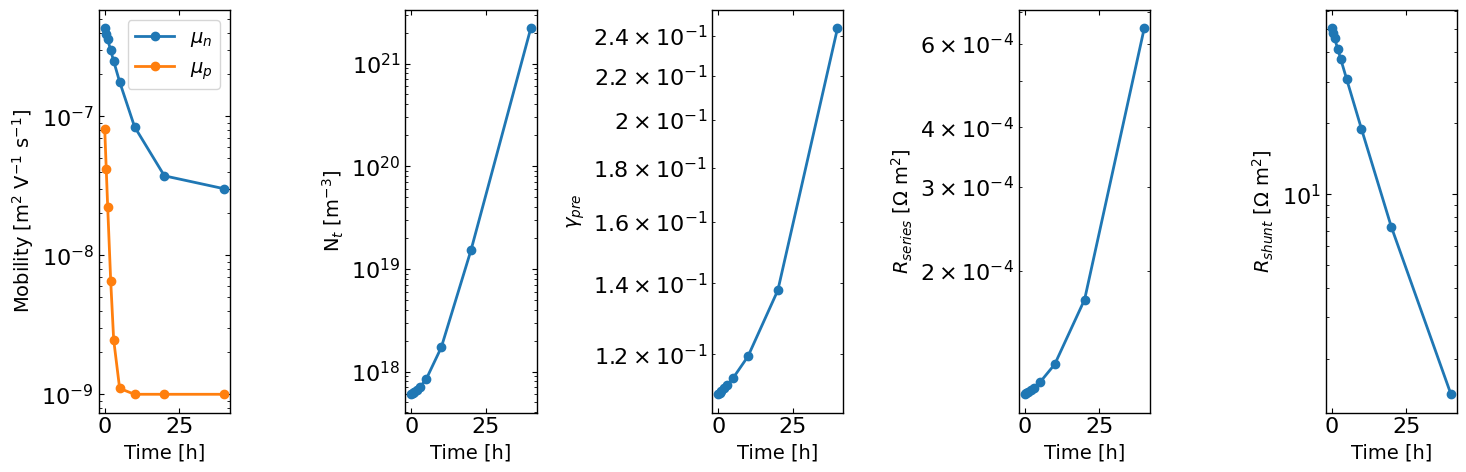
Here we will simulate a degradation type experiment where the hole mobility, bulk trap density, preLangevin factor, series resistance and shunt resistance change over time. We can then investigate how well we can recover the time-dependent parameters and their “Lazy posterior” distributions.
[2]:
times = np.asarray([0, 0.5, 1, 2, 3, 5, 10, 20, 40]) # time points for transient simulations
mun_list  = 4e-7 * np.exp(-times/5) + 3e-8 # time-dependent electron mobility
mup_list  = 8e-8 * np.exp(-times/1.5)**2 + 1e-9 # time-dependent hole mobility
bulk_tr_list = 1e17 * np.exp(times/4) + 5e17 # time-dependent bulk trap density
preLangevin_list = 0.01 * np.exp(times/15) + 0.1 # time-dependent preLangevin factor
R_series_list = 1e-5 * np.exp(times/10) + 1e-4 # time-dependent series resistance
R_shunt_list = 0.5e2 * np.exp(-times/10) + 5e-1 # time-dependent shunt resistance


fig, axes = plt.subplots(1,5, figsize=(15,5))
axes[0].plot(times, mun_list, 'o-')
axes[0].plot(times, mup_list, 'o-')
axes[0].set_yscale('log')
axes[0].set_xlabel('Time [h]')
axes[0].legend([r'$\mu_n$', r'$\mu_p$'])
axes[0].set_ylabel('Mobility [m$^2$ V$^{-1}$ s$^{-1}$]')

axes[1].plot(times, bulk_tr_list, 'o-')
axes[1].set_yscale('log')
axes[1].set_xlabel('Time [h]')
axes[1].set_ylabel(r'N$_t$ [m$^{-3}$]')
axes[2].plot(times, preLangevin_list, 'o-')
axes[2].set_yscale('log')
axes[2].set_xlabel('Time [h]')
axes[2].set_ylabel(r'$\gamma_{pre}$')
axes[3].plot(times, R_series_list, 'o-')
axes[3].set_yscale('log')
axes[3].set_xlabel('Time [h]')
axes[3].set_ylabel(r'$R_{series}$ [$\Omega$ m$^2$]')
axes[4].plot(times, R_shunt_list, 'o-')
axes[4].set_yscale('log')
axes[4].set_xlabel('Time [h]')
axes[4].set_ylabel(r'$R_{shunt}$ [$\Omega$ m$^2$]')
plt.tight_layout()
plt.show()
[3]:
def make_data(times, mun_list, mup_list, bulk_tr_list, preLangevin_list, R_series_list, R_shunt_list):

    # Set the session path for the simulation and the input files
    session_path = os.path.join(os.path.join(os.path.abspath('../'),'SIMsalabim','SimSS'))
    input_path = os.path.join(os.path.join(os.path.join(os.path.abspath('../'),'Data','simsalabim_test_inputs','fakeOPV')))
    simulation_setup_filename = 'simulation_setup_fakeOPV.txt'
    simulation_setup = os.path.join(session_path, simulation_setup_filename)

    # path to the layer files defined in the simulation_setup file
    l1 = 'ZnO.txt'
    l2 = 'ActiveLayer.txt'
    l3 = 'BM_HTL.txt'
    l1 = os.path.join(input_path, l1)
    l2 = os.path.join(input_path, l2)
    l3 = os.path.join(input_path, l3)

    # copy this files to session_path
    force_copy = True
    if not os.path.exists(session_path):
        os.makedirs(session_path)
    for file in [l1,l2,l3,simulation_setup_filename]:
        file = os.path.join(input_path, os.path.basename(file))
        if force_copy or not os.path.exists(os.path.join(session_path, os.path.basename(file))):
            shutil.copyfile(file, os.path.join(session_path, os.path.basename(file)))
        else:
            print('File already exists: ',file)
    dic_res = {}
    print('Generating data for times: ', times)
    for i, t in enumerate(times):
        params = [] # list of parameters to be optimized

        mup = FitParam(name = 'l2.mu_p', value = mup_list[i], bounds = [5e-10,1e-6], log_scale = True, value_type = 'float', fscale = None, rescale = False, display_name=r'$\mu_p$', unit=r'm$^2$ V$^{-1}$s$^{-1}$', axis_type = 'log', force_log = True)
        params.append(mup)

        mun = FitParam(name = 'l2.mu_n', value = mun_list[i], bounds = [5e-10,1e-6], log_scale = True, value_type = 'float', fscale = None, rescale = False, display_name=r'$\mu_n$', unit='m$^2$ V$^{-1}$s$^{-1}$', axis_type = 'log', force_log = True)
        params.append(mun)

        bulk_tr = FitParam(name = 'l2.N_t_bulk', value = bulk_tr_list[i], bounds = [1e17,1e22], log_scale = True, value_type = 'float', fscale = None, rescale = False,  display_name=r'$N_{T}$', unit=r'm$^{-3}$', axis_type = 'log', force_log = True)
        params.append(bulk_tr)

        preLangevin = FitParam(name = 'l2.preLangevin', value = preLangevin_list[i], bounds = [0.005,1], log_scale = True, value_type = 'float', fscale = None, rescale = False, display_name=r'$\gamma_{pre}$', unit=r'-', axis_type = 'log', force_log = True)
        params.append(preLangevin)

        R_series = FitParam(name = 'R_series', value = R_series_list[i], bounds = [1e-5,1e-1], log_scale = True, value_type = 'float', fscale = None, rescale = False,  display_name=r'$R_{series}$', unit=r'$\Omega$ m$^2$', axis_type = 'log', force_log = True)
        params.append(R_series)

        R_shunt = FitParam(name = 'R_shunt', value = R_shunt_list[i], bounds = [1e-2,1e2], log_scale = True, value_type = 'float', fscale = None, rescale = False,  display_name=r'$R_{shunt}$', unit=r'$\Omega$ m$^2$', axis_type = 'log', force_log = True)
        params.append(R_shunt)


        # reset simss
        # Set the JV parameters
        Gfracs = [0.1,0.5,1.0] # Fractions of the generation rate to simulate (None if you want only one light intensity as define in the simulation_setup file)
        UUID = str(uuid.uuid4()) # random UUID to avoid overwriting files

        cmd_pars = [] # see pySIMsalabim documentation for the command line parameters
        # Add the parameters to the command line arguments
        for param in params:
            cmd_pars.append({'par':param.name, 'val':str(param.value)})

        # Run the JV simulation
        ret, mess = run_SS_JV(simulation_setup, session_path, JV_file_name = 'JV.dat', G_fracs = Gfracs, parallel = True, max_jobs = 3, UUID=UUID, cmd_pars=cmd_pars)

        # save data for fitting
        X,y = [],[]
        X_orig,y_orig = [],[]
        if Gfracs is None:
            data = pd.read_csv(os.path.join(session_path, 'JV_'+UUID+'.dat'), sep=r'\s+') # Load the data
            Vext = np.asarray(data['Vext'].values)
            Jext = np.asarray(data['Jext'].values)
            G = np.ones_like(Vext)
            rng = default_rng()#
            noise = rng.standard_normal(Jext.shape) * 0.01 * Jext
            Jext = Jext + noise
            X = Vext
            y = Jext
        else:
            for Gfrac in Gfracs:
                data = pd.read_csv(os.path.join(session_path, 'JV_Gfrac_'+str(Gfrac)+'_'+UUID+'.dat'), sep=r'\s+') # Load the data
                Vext = np.asarray(data['Vext'].values)
                Jext = np.asarray(data['Jext'].values)
                G = np.ones_like(Vext)*Gfrac
                rng = default_rng()#
                noise = 0 #rng.standard_normal(Jext.shape) * 0.005 * Jext

                if len(X) == 0:
                    X = np.vstack((Vext,G)).T
                    y = Jext + noise
                    y_orig = Jext
                else:
                    X = np.vstack((X,np.vstack((Vext,G)).T))
                    y = np.hstack((y,Jext+ noise))
                    y_orig = np.hstack((y_orig,Jext))

            # remove all the current where Jext is higher than a given value
            X = X[y<200]
            X_orig = copy.deepcopy(X)
            y_orig = y_orig[y<200]
            y = y[y<200]

        masks = []
        for Gfrac in Gfracs:
            mask = y[X[:,1]==Gfrac] < 200
            masks.append(mask)

        # Find the minimum number of valid points across all G fractions
        min_points = min(np.sum(mask) for mask in masks)

        # Apply consistent filtering: keep only the first min_points for each G fraction
        X_filtered = []
        y_filtered = []
        y_orig_filtered = []

        for i, Gfrac in enumerate(Gfracs):
            Gfrac_indices = np.where(X[:,1]==Gfrac)[0]
            valid_indices = Gfrac_indices[masks[i]][:min_points]

            X_filtered.append(X[valid_indices])
            y_filtered.append(y[valid_indices])
            y_orig_filtered.append(y_orig[valid_indices])

        X = np.vstack(X_filtered)
        y = np.hstack(y_filtered)
        y_orig = np.hstack(y_orig_filtered)
        X_orig = copy.deepcopy(X)

        # reshape y such that each Gfrac is a column
        y_reshaped = y.reshape((len(Gfracs), int(len(y)/len(Gfracs))))

        # The following calculates sigma using a similar approach as in Eunchi Kim et al. DOI: 10.1002/solr.202500648
        # calculate the sigma for the experimental data
        std_phi = 0.05 # 5% error on light intensity
        std_vol = 0.01 # 10 mV error on voltage

        # get dy/dGfrac
        dJ_dphi = np.gradient(y_reshaped,Gfracs,axis=0,edge_order=2)
        dJ_dV = np.gradient(y_reshaped,X[:,0][X[:,1]==Gfracs[0]],axis=1,edge_order=2)

        phi_term = (std_phi * dJ_dphi)**2
        vol_term = (std_vol * dJ_dV)**2
        phi_term = phi_term.flatten()
        vol_term = vol_term.flatten()
        sigma_J = np.sqrt((std_phi*dJ_dphi)**2 + (std_vol*dJ_dV)**2)
        sigma_J = sigma_J.flatten()  # convert to absolute error

        dic_res[t] = {'X':X, 'y':y, 'sigma_J':sigma_J, 'params':params}

    return dic_res

dic_data = make_data(times, mun_list, mup_list, bulk_tr_list, preLangevin_list, R_series_list, R_shunt_list)
Generating data for times: [ 0. 0.5 1. 2. 3. 5. 10. 20. 40. ]
[4]:
plt.figure()
for _ in dic_data.keys():
    data = dic_data[_]
    X = data['X']
    y = data['y']
    plt.plot(X[X[:,1]==1.0,0],y[X[:,1]==1.0],label='t = '+str(_)+' s, Gfrac = 1.0')
plt.xlabel('Voltage [V]')
plt.ylabel('Current density [A/m$^2$]')
plt.show()

[5]:
# Initialize Ray – ensure this runs only once
if not ray.is_initialized():
    ray.init(ignore_reinit_error=True, num_cpus=180)

@ray.remote
def run_single_chain(params, jv, num_free_params):
    """Run a single optimization chain and return ax_client.summarize()."""

    optimizer = axBOtorchOptimizer(
        params=params,
        agents=jv,
        models=['SOBOL','BOTORCH_MODULAR'],
        n_batches=[5,100],
        batch_size=[5,2],
        ax_client=None,
        max_parallelism=-1,
        model_kwargs_list=get_VMLC_default_model_kwargs_list(
            num_free_params=num_free_params
        ),
        model_gen_kwargs_list=None,
        name='ax_opti',
        parallel=True,
        verbose_logging=False
    )

    optimizer.optimize_turbo(acq_turbo='ts')
    return optimizer.ax_client.summarize()


@ray.remote
def run_single_k(k, entry):
    """Run all optimization for a single dictionary entry (one device)."""

    params      = entry['params']
    X           = entry['X']
    y           = entry['y']
    sigma_J     = entry['sigma_J']
    num_free_params = len([p for p in params if p.type != 'fixed'])

    # ---- Setup SIMsalabim paths ----
    session_path = os.path.join(os.path.abspath('../'), 'SIMsalabim', 'SimSS')
    input_path   = os.path.join(os.path.abspath('../'), 'Data','simsalabim_test_inputs','fakeOPV')

    simulation_setup_filename = 'simulation_setup_fakeOPV.txt'
    simulation_setup = os.path.join(session_path, simulation_setup_filename)

    # ---- Metrics for optimization ----
    metric          = 'nrmse'
    loss            = 'linear'
    tracking_metrics = 'LLH'
    tracking_loss    = 'linear'
    tracking_weight  = 1 / sigma_J**2

    jv = JVAgent(
        params, X, y,
        session_path,
        simulation_setup,
        parallel=True,
        max_jobs=1,
        metric=metric,
        loss=loss,
        tracking_metric=tracking_metrics,
        tracking_loss=tracking_loss,
        tracking_weight=tracking_weight,
        tracking_X=X,
        tracking_y=y,
        tracking_exp_format='JV'
    )

    # ---- Launch 10 optimization chains in parallel ----
    futures = [
        run_single_chain.remote(params, jv, num_free_params)
        for _ in range(10)
    ]

    results = ray.get(futures)

    # Concatenate all dataframes
    data_main = pd.concat(results, ignore_index=True)

    # return a tuple to rebuild the dictionary
    return (k, data_main)


def run_fit(dic):
    """Ray-distributed full optimization over all dictionary entries."""

    futures = [
        run_single_k.remote(k, dic[k])
        for k in dic.keys()
    ]

    results = ray.get(futures)

    # Update dic with results
    for k, data in results:
        dic[k]['data_main'] = data

    return dic
2026-01-20 11:52:39,673 INFO worker.py:2014 -- Started a local Ray instance. View the dashboard at http://127.0.0.1:8265
(run_single_chain pid=1634757) [WARNING 01-20 11:55:45] ax.api.client: Metric IMetric('JV_JV_LLH_linear') not found in optimization config, added as tracking metric.
(run_single_chain pid=1634809) [WARNING 01-20 11:56:15] ax.api.client: Metric IMetric('JV_JV_LLH_linear') not found in optimization config, added as tracking metric.
(run_single_chain pid=1634751) [WARNING 01-20 11:56:34] ax.api.client: Metric IMetric('JV_JV_LLH_linear') not found in optimization config, added as tracking metric.
(run_single_chain pid=1634775) [WARNING 01-20 11:56:44] ax.api.client: Metric IMetric('JV_JV_LLH_linear') not found in optimization config, added as tracking metric.
(run_single_chain pid=1634840) [WARNING 01-20 11:56:51] ax.api.client: Metric IMetric('JV_JV_LLH_linear') not found in optimization config, added as tracking metric.
(run_single_chain pid=1634744) [WARNING 01-20 11:56:58] ax.api.client: Metric IMetric('JV_JV_LLH_linear') not found in optimization config, added as tracking metric. [repeated 3x across cluster] (Ray deduplicates logs by default. Set RAY_DEDUP_LOGS=0 to disable log deduplication, or see https://docs.ray.io/en/master/ray-observability/user-guides/configure-logging.html#log-deduplication for more options.)
(run_single_chain pid=1634801) [WARNING 01-20 11:57:10] ax.api.client: Metric IMetric('JV_JV_LLH_linear') not found in optimization config, added as tracking metric. [repeated 3x across cluster]
(run_single_chain pid=1634802) [WARNING 01-20 11:57:18] ax.api.client: Metric IMetric('JV_JV_LLH_linear') not found in optimization config, added as tracking metric.
(run_single_chain pid=1634805) [WARNING 01-20 11:57:20] ax.api.client: Metric IMetric('JV_JV_LLH_linear') not found in optimization config, added as tracking metric.
(run_single_chain pid=1634760) [WARNING 01-20 11:57:27] ax.api.client: Metric IMetric('JV_JV_LLH_linear') not found in optimization config, added as tracking metric. [repeated 5x across cluster]
(run_single_chain pid=1634784) [WARNING 01-20 11:57:39] ax.api.client: Metric IMetric('JV_JV_LLH_linear') not found in optimization config, added as tracking metric. [repeated 2x across cluster]
(run_single_chain pid=1634803) [WARNING 01-20 11:57:46] ax.api.client: Metric IMetric('JV_JV_LLH_linear') not found in optimization config, added as tracking metric. [repeated 4x across cluster]
(run_single_chain pid=1634796) [ERROR 01-20 11:58:06] optimpv.axBOtorchOptimizer: Error in Turbo batch 83: All attempts to fit the model have failed.
(run_single_chain pid=1634796) [ERROR 01-20 11:58:06] optimpv.axBOtorchOptimizer: We are stopping the optimization process
(run_single_chain pid=1634796) [WARNING 01-20 11:58:06] ax.api.client: Metric IMetric('JV_JV_LLH_linear') not found in optimization config, added as tracking metric.
(run_single_chain pid=1634839) [WARNING 01-20 11:58:07] ax.api.client: Metric IMetric('JV_JV_LLH_linear') not found in optimization config, added as tracking metric.
(run_single_chain pid=1634814) [WARNING 01-20 11:58:14] ax.api.client: Metric IMetric('JV_JV_LLH_linear') not found in optimization config, added as tracking metric. [repeated 3x across cluster]
(run_single_chain pid=1634756) [WARNING 01-20 11:58:25] ax.api.client: Metric IMetric('JV_JV_LLH_linear') not found in optimization config, added as tracking metric. [repeated 3x across cluster]
(run_single_chain pid=1634770) [WARNING 01-20 11:58:35] ax.api.client: Metric IMetric('JV_JV_LLH_linear') not found in optimization config, added as tracking metric. [repeated 2x across cluster]
(run_single_chain pid=1634748) [WARNING 01-20 11:58:42] ax.api.client: Metric IMetric('JV_JV_LLH_linear') not found in optimization config, added as tracking metric. [repeated 2x across cluster]
(run_single_chain pid=1634824) [WARNING 01-20 11:58:47] ax.api.client: Metric IMetric('JV_JV_LLH_linear') not found in optimization config, added as tracking metric.
(run_single_chain pid=1634806) [WARNING 01-20 11:58:49] ax.api.client: Metric IMetric('JV_JV_LLH_linear') not found in optimization config, added as tracking metric.
(run_single_chain pid=1634798) [WARNING 01-20 11:58:58] ax.api.client: Metric IMetric('JV_JV_LLH_linear') not found in optimization config, added as tracking metric. [repeated 5x across cluster]
(run_single_chain pid=1634792) [WARNING 01-20 11:59:03] ax.api.client: Metric IMetric('JV_JV_LLH_linear') not found in optimization config, added as tracking metric. [repeated 3x across cluster]
(run_single_chain pid=1634746) [WARNING 01-20 11:59:09] ax.api.client: Metric IMetric('JV_JV_LLH_linear') not found in optimization config, added as tracking metric. [repeated 4x across cluster]
(run_single_chain pid=1634754) [WARNING 01-20 11:59:20] ax.api.client: Metric IMetric('JV_JV_LLH_linear') not found in optimization config, added as tracking metric. [repeated 2x across cluster]
(run_single_chain pid=1634750) [WARNING 01-20 11:59:27] ax.api.client: Metric IMetric('JV_JV_LLH_linear') not found in optimization config, added as tracking metric. [repeated 8x across cluster]
(run_single_chain pid=1634808) [WARNING 01-20 11:59:32] ax.api.client: Metric IMetric('JV_JV_LLH_linear') not found in optimization config, added as tracking metric. [repeated 5x across cluster]
(run_single_chain pid=1634734) [WARNING 01-20 11:59:37] ax.api.client: Metric IMetric('JV_JV_LLH_linear') not found in optimization config, added as tracking metric. [repeated 5x across cluster]
(run_single_chain pid=1634733) [WARNING 01-20 11:59:49] ax.api.client: Metric IMetric('JV_JV_LLH_linear') not found in optimization config, added as tracking metric. [repeated 5x across cluster]
(run_single_chain pid=1634743) [WARNING 01-20 11:59:55] ax.api.client: Metric IMetric('JV_JV_LLH_linear') not found in optimization config, added as tracking metric.
(run_single_chain pid=1634795) [WARNING 01-20 11:59:58] ax.api.client: Metric IMetric('JV_JV_LLH_linear') not found in optimization config, added as tracking metric.
(run_single_chain pid=1634817) [WARNING 01-20 12:00:04] ax.api.client: Metric IMetric('JV_JV_LLH_linear') not found in optimization config, added as tracking metric. [repeated 5x across cluster]
(run_single_chain pid=1634819) [WARNING 01-20 12:00:14] ax.api.client: Metric IMetric('JV_JV_LLH_linear') not found in optimization config, added as tracking metric. [repeated 6x across cluster]
(run_single_chain pid=1634843) [WARNING 01-20 12:00:27] ax.api.client: Metric IMetric('JV_JV_LLH_linear') not found in optimization config, added as tracking metric. [repeated 2x across cluster]
[6]:
%%time
dic_data = run_fit(dic_data)
CPU times: user 3.41 s, sys: 1.21 s, total: 4.62 s
Wall time: 7min 46s
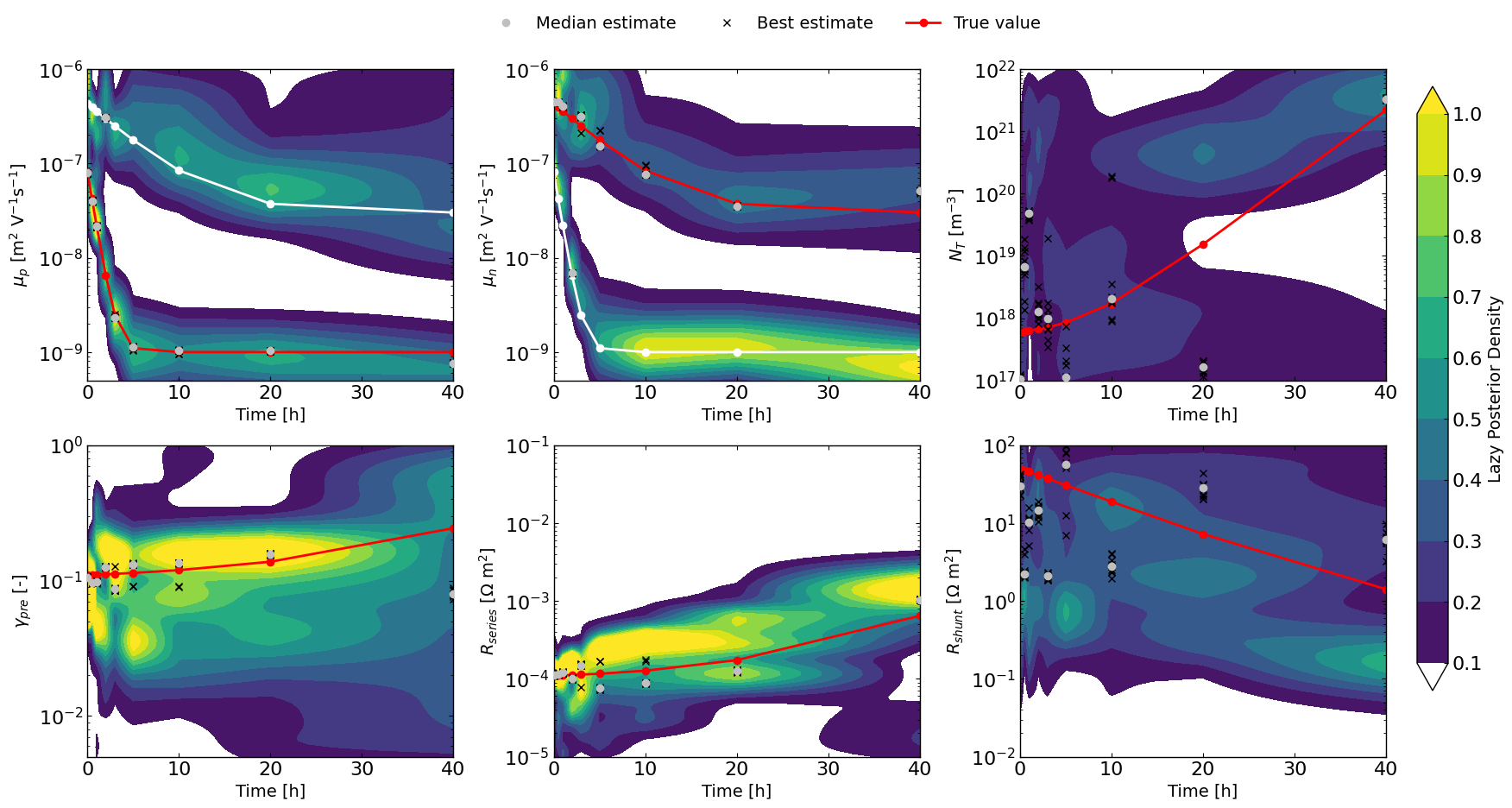
The “lazy” posterior
The following implementation has NO mathematical support as far as I (VMLC) knows, but I will make the following argument.
One could think of each Bayesian Optimization run using TuRBO as similar to a different chain in a classical MCMC approach.
In that analogy, the random sampling first step for the BO would be equivalent to the warm-up stage in MCMC which can therefore be discarded. The TURBO stage would be equivalent to the normal chain path.
Therefore if we were to looks at the density of point that gets explored during the TURBO stage for multiple “chains” we would expect to get something that is not too different from doing MCMC.
To explore this, the LazyPosterior class has been implemented and shows promising results.
[7]:
from optimpv.posterior.lazy_posterior import LazyPosterior

viridis = plt.get_cmap('viridis', len(dic_data.keys()))

fig, axes = plt.subplots(2,3, figsize=(18,10))
ax_ = axes.flatten()
for idx_par in range(len(dic_data[0]['params'])):  # 0: mup, 1: mun, 2: bulk_tr, 3: preLangevin, 4: R_series, 5: R_shunt
    kde_2d = []
    median_pars,top10 = [], []
    for _ in dic_data.keys():
        outcome_name = 'JV_JV_LLH_linear' #optimizer.all_tracking_metrics[0] #'LLH'
        data_main = dic_data[_]['data_main']
        data_main = data_main[data_main['trial_index']>=30] # discard the random sampling part
        params = dic_data[_]['params']
        lazy_post = LazyPosterior(params, data_main, outcome_name)
        par_name = params[idx_par].name
        par_log_scale = params[idx_par].log_scale or params[idx_par].force_log
        kde_ = lazy_post._compute_1D_kde(par_name, log_scale=par_log_scale)
        params_median = lazy_post.get_top_n_metrics_params('median', num=10)
        top10_params = lazy_post.get_top_n_best_params(num=10)
        top10.append([val[idx_par].value for val in top10_params])

        # calculate the median of the top 10 params
        median_pars.append(params_median[idx_par].value)
        bounds = params[idx_par].bounds
        if par_log_scale:
            par_x = np.logspace(np.log10(bounds[0]), np.log10(bounds[1]), 100)
        else:
            par_x = np.linspace(bounds[0], bounds[1], 100)

        kde_2d.append((par_x,kde_(par_x)))

    # make a grid for times
    times_grid = np.array(list(dic_data.keys()))
    X_, Y_ = np.meshgrid(times_grid, kde_2d[0][0])
    Z = np.zeros_like(X_)
    for i, t in enumerate(times_grid):
        kde_vals = kde_2d[i][1]
        Z[:,i] = kde_vals


    # Choose a base colormap
    vmin = 0.1
    vmax = 1.0
    cmap = matplotlib.colormaps.get_cmap('viridis').copy()

    # Set the color for values below the threshold
    cmap.set_under("white")
    # last viridis color for values above vmax
    cmap.set_over(cmap.colors[-1])

    # Levels: start at threshold
    levels = np.linspace(vmin, vmax, 10)
    cp = ax_[idx_par].contourf(X_, Y_, Z, levels=levels, cmap=cmap,extend='both')
    ax_[idx_par].plot(times, median_pars, 'o', color='silver', label='Median estimate',zorder=6)
    top10=np.asarray(top10)
    for i in range(len(times)):
        ax_[idx_par].plot(times, top10[:,i], 'x', color='black', label='Best estimate' if i == 0 else "",zorder=4)
    if idx_par == 1 or idx_par == 0:
        ax_[idx_par].plot(times, mun_list, 'w-o' if idx_par==0 else 'r-o', label=r'$\mu_n$ true')
        ax_[idx_par].plot(times, mup_list, 'w-o' if idx_par==1 else 'r-o', label=r'$\mu_p$ true')

    else:
        true_vals = {
            2: bulk_tr_list,
            3: preLangevin_list,
            4: R_series_list,
            5: R_shunt_list
        }
        ax_[idx_par].plot(times, true_vals[idx_par], 'r-o', label='True value')

    ax_[idx_par].set_ylim(bounds)
    # plt.colorbar(cp, ax=ax_[idx_par])
    ax_[idx_par].set_xlabel('Time [h]')
    ax_[idx_par].set_ylabel(params[idx_par].full_name)
    ax_[idx_par].set_yscale('log' if params[idx_par].log_scale or params[idx_par].force_log else 'linear')
# set one main colorbar for all subplots
plt.tight_layout()
fig.subplots_adjust(right=0.9, top=0.87)
cbar_ax = fig.add_axes([0.92, 0.15, 0.02, 0.7])
cbar = fig.colorbar(cp, cax=cbar_ax)
cbar.set_label('Lazy Posterior Density')
# add one legend for all subplots
handles, labels = ax_[-1].get_legend_handles_labels()
fig.legend(handles, labels, loc='upper center', bbox_to_anchor=(0.5, 0.95), ncol=3,frameon=False)

plt.show()
[8]:
# Clean up the output files (comment out if you want to keep the output files)
sim.clean_all_output(session_path)
sim.delete_folders('tmp',session_path)
# uncomment the following lines to delete specific files
sim.clean_up_output('ZnO',session_path)
sim.clean_up_output('ActiveLayer',session_path)
sim.clean_up_output('BM_HTL',session_path)
sim.clean_up_output('simulation_setup_fakeOPV',session_path)