Fit non ideal diode equation to dark or light JV-curve
using the solving method described in Solid-State Electronics 44 (2000) 1861-1864.
For light:
using the solving method described in Solar Energy Materials & Solar Cells 81 (2004) 269–277.
[6]:
# Import necessary libraries
import warnings, os, sys, torch, copy
# remove warnings from the output
os.environ["PYTHONWARNINGS"] = "ignore"
warnings.filterwarnings(action='ignore', category=FutureWarning)
warnings.filterwarnings(action='ignore', category=UserWarning)
import pandas as pd
import matplotlib.pyplot as plt
import numpy as np
from copy import deepcopy
import ax, logging
from ax.utils.notebook.plotting import init_notebook_plotting
init_notebook_plotting() # for Jupyter notebooks
try:
from optimpv import *
from optimpv.optimizers.axBOtorch.axUtils import *
from optimpv.models.Diodefits.DiodeAgent import DiodeAgent
from optimpv.models.Diodefits.DiodeModel import *
except Exception as e:
sys.path.append('../') # add the path to the optimpv module
from optimpv import *
from optimpv.optimizers.axBOtorch.axUtils import *
from optimpv.models.Diodefits.DiodeAgent import DiodeAgent
from optimpv.models.Diodefits.DiodeModel import *
Define the parameters for the simulation
[7]:
params = []
J0 = FitParam(name = 'J0', value = 1e-5, bounds = [1e-6,1e-3], log_scale = True, rescale = False, value_type = 'float', type='range', display_name=r'$J_0$', unit='A m$^{-2}$', axis_type = 'log',force_log=True)
params.append(J0)
n = FitParam(name = 'n', value = 1.5, bounds = [1,2], log_scale = False, value_type = 'float', type='range', display_name=r'$n$', unit='', axis_type = 'linear')
params.append(n)
R_series = FitParam(name = 'R_series', value = 1e-4, bounds = [1e-5,1e-3], log_scale = True, rescale = False, value_type = 'float', type='range', display_name=r'$R_{\text{series}}$', unit=r'$\Omega$ m$^2$', axis_type = 'log',force_log=True)
params.append(R_series)
R_shunt = FitParam(name = 'R_shunt', value = 1e-1, bounds = [1e-2,1e2], log_scale = True, rescale = False, value_type = 'float', type='range', display_name=r'$R_{\text{shunt}}$', unit=r'$\Omega$ m$^2$', axis_type = 'log',force_log=True)
params.append(R_shunt)
# original values
params_orig = copy.deepcopy(params)
num_free_params = len([p for p in params if p.type != 'fixed'])
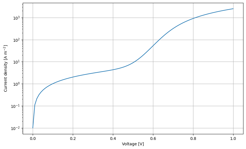
Generate some fake data for the dark JV
[8]:
# Create JV to fit
X = np.linspace(0.001,1,100)
y = NonIdealDiode_dark(X, J0.value, n.value, R_series.value, R_shunt.value)
plt.figure(figsize=(10,6))
plt.semilogy(X,y)
plt.xlabel('Voltage [V]')
plt.ylabel('Current density [A m$^{-2}$]')
plt.grid()
plt.show()
Run the optimization
While very inefficient we first try to fit the data using Bayesian optimization, then we use scipy.optimize.minize to demonstrate the difference in speed and accuracy.
[9]:
# Define the Agent and the target metric/loss function
metric = 'mse' # can be 'nrmse', 'mse', 'mae'
loss = 'soft_l1' # can be 'linear', 'huber', 'soft_l1'
exp_format = 'dark' # can be 'dark', 'light' depending on the type of data you have
use_pvlib = False # if True, use pvlib to calculate the diode model if not use the implementation in DiodeModel.py
diode = DiodeAgent(params, X, y, metric = metric, loss = loss, minimize=True,exp_format=exp_format,use_pvlib=use_pvlib,transforms='log')
First with BO
[10]:
from optimpv.optimizers.axBOtorch.axBOtorchOptimizer import axBOtorchOptimizer
from optimpv.optimizers.axBOtorch.axUtils import get_VMLC_default_model_kwargs_list
# Define the optimizer
optimizer = axBOtorchOptimizer(params = params, agents = diode, models = ['SOBOL','BOTORCH_MODULAR'],n_batches = [1,20], batch_size = [10,2], model_kwargs_list = get_VMLC_default_model_kwargs_list(num_free_params))
[11]:
optimizer.optimize() # run the optimization with ax
[INFO 01-20 10:22:57] optimpv.axBOtorchOptimizer: Trial 0 with parameters: {'J0': -4.590295686386526, 'n': 1.3030478302389383, 'R_series': -4.0192861668765545, 'R_shunt': -0.2137989103794098}
[INFO 01-20 10:22:57] optimpv.axBOtorchOptimizer: Trial 1 with parameters: {'J0': -3.8798954794183373, 'n': 1.797770595178008, 'R_series': -3.373800491914153, 'R_shunt': 1.969033159315586}
[INFO 01-20 10:22:57] optimpv.axBOtorchOptimizer: Trial 2 with parameters: {'J0': -3.6398436930030584, 'n': 1.0774983577430248, 'R_series': -4.997814267873764, 'R_shunt': -1.839151106774807}
[INFO 01-20 10:22:57] optimpv.axBOtorchOptimizer: Trial 3 with parameters: {'J0': -5.932276636362076, 'n': 1.5721562951803207, 'R_series': -3.6413318384438753, 'R_shunt': 0.09563562273979187}
[INFO 01-20 10:22:57] optimpv.axBOtorchOptimizer: Trial 4 with parameters: {'J0': -5.413540933281183, 'n': 1.1635781843215227, 'R_series': -3.188526190817356, 'R_shunt': 0.8831532523036003}
[INFO 01-20 10:22:57] optimpv.axBOtorchOptimizer: Trial 5 with parameters: {'J0': -3.015634970739484, 'n': 1.6574474554508924, 'R_series': -4.418423840776086, 'R_shunt': -1.174794927239418}
[INFO 01-20 10:22:57] optimpv.axBOtorchOptimizer: Trial 6 with parameters: {'J0': -4.463082876987755, 'n': 1.4673179872334003, 'R_series': -3.7963324673473835, 'R_shunt': 1.0097547620534897}
[INFO 01-20 10:22:57] optimpv.axBOtorchOptimizer: Trial 7 with parameters: {'J0': -5.068021464161575, 'n': 1.9611223712563515, 'R_series': -4.5644971411675215, 'R_shunt': -0.800144262611866}
[INFO 01-20 10:22:57] optimpv.axBOtorchOptimizer: Trial 8 with parameters: {'J0': -4.890716157853603, 'n': 1.0421880148351192, 'R_series': -3.9631383400410414, 'R_shunt': -1.3079106882214546}
[INFO 01-20 10:22:57] optimpv.axBOtorchOptimizer: Trial 9 with parameters: {'J0': -4.288617102429271, 'n': 1.5444782972335815, 'R_series': -4.678934592753649, 'R_shunt': 0.5018647164106369}
[INFO 01-20 10:22:58] optimpv.axBOtorchOptimizer: Trial 0 completed with results: {'diode_dark_mse_soft_l1': 0.36320387540912913}
[INFO 01-20 10:22:58] optimpv.axBOtorchOptimizer: Trial 1 completed with results: {'diode_dark_mse_soft_l1': 1.4796490471554749}
[INFO 01-20 10:22:58] optimpv.axBOtorchOptimizer: Trial 2 completed with results: {'diode_dark_mse_soft_l1': 1.833797664789261}
[INFO 01-20 10:22:58] optimpv.axBOtorchOptimizer: Trial 3 completed with results: {'diode_dark_mse_soft_l1': 0.8353462325944268}
[INFO 01-20 10:22:58] optimpv.axBOtorchOptimizer: Trial 4 completed with results: {'diode_dark_mse_soft_l1': 0.9511062518273605}
[INFO 01-20 10:22:58] optimpv.axBOtorchOptimizer: Trial 5 completed with results: {'diode_dark_mse_soft_l1': 0.39896494804175564}
[INFO 01-20 10:22:58] optimpv.axBOtorchOptimizer: Trial 6 completed with results: {'diode_dark_mse_soft_l1': 0.9707791004639157}
[INFO 01-20 10:22:58] optimpv.axBOtorchOptimizer: Trial 7 completed with results: {'diode_dark_mse_soft_l1': 0.4570247056653227}
[INFO 01-20 10:22:58] optimpv.axBOtorchOptimizer: Trial 8 completed with results: {'diode_dark_mse_soft_l1': 0.5612974136735662}
[INFO 01-20 10:22:58] optimpv.axBOtorchOptimizer: Trial 9 completed with results: {'diode_dark_mse_soft_l1': 0.7431945823058039}
[INFO 01-20 10:22:59] optimpv.axBOtorchOptimizer: Trial 10 with parameters: {'J0': -5.517787627962182, 'n': 2.0, 'R_series': -4.25174363617085, 'R_shunt': -0.5143063472736211}
[INFO 01-20 10:22:59] optimpv.axBOtorchOptimizer: Trial 11 with parameters: {'J0': -5.8957545857578655, 'n': 1.3037505297274097, 'R_series': -4.267829424269869, 'R_shunt': -0.30774076088429103}
[INFO 01-20 10:23:00] optimpv.axBOtorchOptimizer: Trial 10 completed with results: {'diode_dark_mse_soft_l1': 0.9266565586387903}
[INFO 01-20 10:23:00] optimpv.axBOtorchOptimizer: Trial 11 completed with results: {'diode_dark_mse_soft_l1': 0.22936450030754152}
[INFO 01-20 10:23:00] optimpv.axBOtorchOptimizer: Trial 12 with parameters: {'J0': -5.941769579760871, 'n': 1.3583704213788943, 'R_series': -4.198188078474639, 'R_shunt': -0.9652523507557}
[INFO 01-20 10:23:00] optimpv.axBOtorchOptimizer: Trial 13 with parameters: {'J0': -4.6566742158905665, 'n': 1.0765879425564462, 'R_series': -4.209374753856531, 'R_shunt': 0.18802652820298293}
[INFO 01-20 10:23:00] optimpv.axBOtorchOptimizer: Trial 12 completed with results: {'diode_dark_mse_soft_l1': 0.010908967222543087}
[INFO 01-20 10:23:00] optimpv.axBOtorchOptimizer: Trial 13 completed with results: {'diode_dark_mse_soft_l1': 0.9184662947916995}
[INFO 01-20 10:23:01] optimpv.axBOtorchOptimizer: Trial 14 with parameters: {'J0': -6.0, 'n': 1.4148292483546656, 'R_series': -4.122529840648361, 'R_shunt': -2.0}
[INFO 01-20 10:23:01] optimpv.axBOtorchOptimizer: Trial 15 with parameters: {'J0': -6.0, 'n': 1.49226647734498, 'R_series': -4.274291811297386, 'R_shunt': -1.418145241469296}
[INFO 01-20 10:23:01] optimpv.axBOtorchOptimizer: Trial 14 completed with results: {'diode_dark_mse_soft_l1': 0.45212157172342815}
[INFO 01-20 10:23:01] optimpv.axBOtorchOptimizer: Trial 15 completed with results: {'diode_dark_mse_soft_l1': 0.12771787497658327}
[INFO 01-20 10:23:02] optimpv.axBOtorchOptimizer: Trial 16 with parameters: {'J0': -6.0, 'n': 1.455720470756373, 'R_series': -4.218228885649684, 'R_shunt': -0.8001556204327795}
[INFO 01-20 10:23:02] optimpv.axBOtorchOptimizer: Trial 17 with parameters: {'J0': -6.0, 'n': 1.408768533375016, 'R_series': -4.322717780797796, 'R_shunt': -0.9530332925295997}
[INFO 01-20 10:23:02] optimpv.axBOtorchOptimizer: Trial 16 completed with results: {'diode_dark_mse_soft_l1': 0.0956306315401001}
[INFO 01-20 10:23:02] optimpv.axBOtorchOptimizer: Trial 17 completed with results: {'diode_dark_mse_soft_l1': 0.03441319612876104}
[INFO 01-20 10:23:02] optimpv.axBOtorchOptimizer: Trial 18 with parameters: {'J0': -4.058870871072208, 'n': 1.3683472660817682, 'R_series': -4.237920791497144, 'R_shunt': -1.0186577054841774}
[INFO 01-20 10:23:02] optimpv.axBOtorchOptimizer: Trial 19 with parameters: {'J0': -6.0, 'n': 2.0, 'R_series': -5.0, 'R_shunt': -1.7968829500179053}
[INFO 01-20 10:23:02] optimpv.axBOtorchOptimizer: Trial 18 completed with results: {'diode_dark_mse_soft_l1': 0.3425592998191629}
[INFO 01-20 10:23:02] optimpv.axBOtorchOptimizer: Trial 19 completed with results: {'diode_dark_mse_soft_l1': 0.637732699605754}
[INFO 01-20 10:23:03] optimpv.axBOtorchOptimizer: Trial 20 with parameters: {'J0': -6.0, 'n': 1.6193345071233862, 'R_series': -4.6245010980028285, 'R_shunt': -1.0314495090753026}
[INFO 01-20 10:23:03] optimpv.axBOtorchOptimizer: Trial 21 with parameters: {'J0': -6.0, 'n': 1.3131987289006801, 'R_series': -4.020564839046849, 'R_shunt': -0.913343944452667}
[INFO 01-20 10:23:03] optimpv.axBOtorchOptimizer: Trial 20 completed with results: {'diode_dark_mse_soft_l1': 0.22321719333855627}
[INFO 01-20 10:23:03] optimpv.axBOtorchOptimizer: Trial 21 completed with results: {'diode_dark_mse_soft_l1': 0.0063698978641171244}
[INFO 01-20 10:23:04] optimpv.axBOtorchOptimizer: Trial 22 with parameters: {'J0': -5.13966313845696, 'n': 1.4708440392878115, 'R_series': -3.0, 'R_shunt': -1.00774067792918}
[INFO 01-20 10:23:04] optimpv.axBOtorchOptimizer: Trial 23 with parameters: {'J0': -3.6451253896460667, 'n': 2.0, 'R_series': -3.0, 'R_shunt': -1.4457977359070595}
[INFO 01-20 10:23:04] optimpv.axBOtorchOptimizer: Trial 22 completed with results: {'diode_dark_mse_soft_l1': 0.19610681347110592}
[INFO 01-20 10:23:04] optimpv.axBOtorchOptimizer: Trial 23 completed with results: {'diode_dark_mse_soft_l1': 0.3223937222682829}
[INFO 01-20 10:23:05] optimpv.axBOtorchOptimizer: Trial 24 with parameters: {'J0': -5.308880254628436, 'n': 1.4318158852750458, 'R_series': -4.317068348309042, 'R_shunt': -1.0013619790123305}
[INFO 01-20 10:23:05] optimpv.axBOtorchOptimizer: Trial 25 with parameters: {'J0': -3.5371934250028563, 'n': 2.0, 'R_series': -5.0, 'R_shunt': -1.2832742526257515}
[INFO 01-20 10:23:05] optimpv.axBOtorchOptimizer: Trial 24 completed with results: {'diode_dark_mse_soft_l1': 0.020007101258522564}
[INFO 01-20 10:23:05] optimpv.axBOtorchOptimizer: Trial 25 completed with results: {'diode_dark_mse_soft_l1': 0.08086507884332583}
[INFO 01-20 10:23:06] optimpv.axBOtorchOptimizer: Trial 26 with parameters: {'J0': -6.0, 'n': 1.264990155988061, 'R_series': -5.0, 'R_shunt': -1.0151490045870775}
[INFO 01-20 10:23:06] optimpv.axBOtorchOptimizer: Trial 27 with parameters: {'J0': -3.0, 'n': 2.0, 'R_series': -5.0, 'R_shunt': -0.622054858928418}
[INFO 01-20 10:23:06] optimpv.axBOtorchOptimizer: Trial 26 completed with results: {'diode_dark_mse_soft_l1': 0.23398550355684655}
[INFO 01-20 10:23:06] optimpv.axBOtorchOptimizer: Trial 27 completed with results: {'diode_dark_mse_soft_l1': 0.16799613074816344}
[INFO 01-20 10:23:06] optimpv.axBOtorchOptimizer: Trial 28 with parameters: {'J0': -5.619786685706408, 'n': 1.3434007291486076, 'R_series': -3.913528772664132, 'R_shunt': -1.0030014921286132}
[INFO 01-20 10:23:06] optimpv.axBOtorchOptimizer: Trial 29 with parameters: {'J0': -6.0, 'n': 1.1123058193598212, 'R_series': -3.0, 'R_shunt': -0.98236416319798}
[INFO 01-20 10:23:06] optimpv.axBOtorchOptimizer: Trial 28 completed with results: {'diode_dark_mse_soft_l1': 0.0018222496383164533}
[INFO 01-20 10:23:06] optimpv.axBOtorchOptimizer: Trial 29 completed with results: {'diode_dark_mse_soft_l1': 0.13293016075558972}
[INFO 01-20 10:23:07] optimpv.axBOtorchOptimizer: Trial 30 with parameters: {'J0': -3.0, 'n': 2.0, 'R_series': -4.100186242074418, 'R_shunt': -1.0587058671997123}
[INFO 01-20 10:23:07] optimpv.axBOtorchOptimizer: Trial 31 with parameters: {'J0': -3.0, 'n': 2.0, 'R_series': -4.152638153704934, 'R_shunt': -2.0}
[INFO 01-20 10:23:07] optimpv.axBOtorchOptimizer: Trial 30 completed with results: {'diode_dark_mse_soft_l1': 0.030242965404738698}
[INFO 01-20 10:23:07] optimpv.axBOtorchOptimizer: Trial 31 completed with results: {'diode_dark_mse_soft_l1': 0.48666720192704194}
[INFO 01-20 10:23:08] optimpv.axBOtorchOptimizer: Trial 32 with parameters: {'J0': -3.6597854877904306, 'n': 1.8981516739797706, 'R_series': -4.242615255070308, 'R_shunt': -1.005079816072798}
[INFO 01-20 10:23:08] optimpv.axBOtorchOptimizer: Trial 33 with parameters: {'J0': -3.0, 'n': 1.8912181892453483, 'R_series': -3.0003277073716537, 'R_shunt': -0.425734715272033}
[INFO 01-20 10:23:08] optimpv.axBOtorchOptimizer: Trial 32 completed with results: {'diode_dark_mse_soft_l1': 0.0030852585244764974}
[INFO 01-20 10:23:08] optimpv.axBOtorchOptimizer: Trial 33 completed with results: {'diode_dark_mse_soft_l1': 0.2409247983639644}
[INFO 01-20 10:23:09] optimpv.axBOtorchOptimizer: Trial 34 with parameters: {'J0': -3.447249073669112, 'n': 2.0, 'R_series': -4.2774010615071125, 'R_shunt': -1.0107549668246034}
[INFO 01-20 10:23:09] optimpv.axBOtorchOptimizer: Trial 35 with parameters: {'J0': -4.3793345698052715, 'n': 1.6865705343948572, 'R_series': -4.199913627729149, 'R_shunt': -1.0304701924539534}
[INFO 01-20 10:23:09] optimpv.axBOtorchOptimizer: Trial 34 completed with results: {'diode_dark_mse_soft_l1': 0.004958984730179861}
[INFO 01-20 10:23:09] optimpv.axBOtorchOptimizer: Trial 35 completed with results: {'diode_dark_mse_soft_l1': 0.0030695237285360832}
[INFO 01-20 10:23:10] optimpv.axBOtorchOptimizer: Trial 36 with parameters: {'J0': -4.128059384924242, 'n': 1.8159263176581928, 'R_series': -4.337234009668701, 'R_shunt': -1.2131533340859166}
[INFO 01-20 10:23:10] optimpv.axBOtorchOptimizer: Trial 37 with parameters: {'J0': -3.9698756377704205, 'n': 1.7419096949680588, 'R_series': -3.977862325783504, 'R_shunt': -0.885913736922967}
[INFO 01-20 10:23:10] optimpv.axBOtorchOptimizer: Trial 36 completed with results: {'diode_dark_mse_soft_l1': 0.03038379175520811}
[INFO 01-20 10:23:10] optimpv.axBOtorchOptimizer: Trial 37 completed with results: {'diode_dark_mse_soft_l1': 0.006141867041105087}
[INFO 01-20 10:23:11] optimpv.axBOtorchOptimizer: Trial 38 with parameters: {'J0': -4.844851227624488, 'n': 1.5476970470113571, 'R_series': -4.045480329531854, 'R_shunt': -0.9819340210116745}
[INFO 01-20 10:23:11] optimpv.axBOtorchOptimizer: Trial 39 with parameters: {'J0': -6.0, 'n': 1.2765063790595126, 'R_series': -3.8825564316801175, 'R_shunt': -1.027822637854083}
[INFO 01-20 10:23:11] optimpv.axBOtorchOptimizer: Trial 38 completed with results: {'diode_dark_mse_soft_l1': 0.00042324589022113557}
[INFO 01-20 10:23:11] optimpv.axBOtorchOptimizer: Trial 39 completed with results: {'diode_dark_mse_soft_l1': 0.0022572368002427012}
[INFO 01-20 10:23:12] optimpv.axBOtorchOptimizer: Trial 40 with parameters: {'J0': -4.126966675088232, 'n': 1.7302605697486602, 'R_series': -4.312464726075406, 'R_shunt': -0.8988449316398102}
[INFO 01-20 10:23:12] optimpv.axBOtorchOptimizer: Trial 41 with parameters: {'J0': -4.250310596243449, 'n': 1.6801568455969793, 'R_series': -3.8995585029682025, 'R_shunt': -1.023128915269654}
[INFO 01-20 10:23:12] optimpv.axBOtorchOptimizer: Trial 40 completed with results: {'diode_dark_mse_soft_l1': 0.011287242566982325}
[INFO 01-20 10:23:12] optimpv.axBOtorchOptimizer: Trial 41 completed with results: {'diode_dark_mse_soft_l1': 0.004380178052649342}
[INFO 01-20 10:23:13] optimpv.axBOtorchOptimizer: Trial 42 with parameters: {'J0': -4.478207462118201, 'n': 1.6249590051819887, 'R_series': -4.045851571407573, 'R_shunt': -0.929756170174308}
[INFO 01-20 10:23:13] optimpv.axBOtorchOptimizer: Trial 43 with parameters: {'J0': -3.5260348525360623, 'n': 1.8907700595825256, 'R_series': -4.050247134851102, 'R_shunt': -0.9333349311241541}
[INFO 01-20 10:23:13] optimpv.axBOtorchOptimizer: Trial 42 completed with results: {'diode_dark_mse_soft_l1': 0.001959761077015454}
[INFO 01-20 10:23:13] optimpv.axBOtorchOptimizer: Trial 43 completed with results: {'diode_dark_mse_soft_l1': 0.004135199919126364}
[INFO 01-20 10:23:14] optimpv.axBOtorchOptimizer: Trial 44 with parameters: {'J0': -5.442161486504113, 'n': 1.4138706937119372, 'R_series': -4.0042292595357365, 'R_shunt': -1.0019552363532265}
[INFO 01-20 10:23:14] optimpv.axBOtorchOptimizer: Trial 45 with parameters: {'J0': -6.0, 'n': 1.2365308526311758, 'R_series': -3.887316113785582, 'R_shunt': -0.9142943443804525}
[INFO 01-20 10:23:14] optimpv.axBOtorchOptimizer: Trial 44 completed with results: {'diode_dark_mse_soft_l1': 0.00030656741921442077}
[INFO 01-20 10:23:14] optimpv.axBOtorchOptimizer: Trial 45 completed with results: {'diode_dark_mse_soft_l1': 0.015124280170036641}
[INFO 01-20 10:23:15] optimpv.axBOtorchOptimizer: Trial 46 with parameters: {'J0': -3.968482876729027, 'n': 1.7847116736772404, 'R_series': -4.0754200945016565, 'R_shunt': -0.9878271207576887}
[INFO 01-20 10:23:15] optimpv.axBOtorchOptimizer: Trial 47 with parameters: {'J0': -5.766214462091758, 'n': 1.3455919463232846, 'R_series': -4.00658095278114, 'R_shunt': -1.0184403240065314}
[INFO 01-20 10:23:15] optimpv.axBOtorchOptimizer: Trial 46 completed with results: {'diode_dark_mse_soft_l1': 0.0012097390826957266}
[INFO 01-20 10:23:15] optimpv.axBOtorchOptimizer: Trial 47 completed with results: {'diode_dark_mse_soft_l1': 0.0008885809851602033}
[INFO 01-20 10:23:16] optimpv.axBOtorchOptimizer: Trial 48 with parameters: {'J0': -4.660637570952288, 'n': 1.5863609248994193, 'R_series': -4.056858026474981, 'R_shunt': -1.067384006691599}
[INFO 01-20 10:23:16] optimpv.axBOtorchOptimizer: Trial 49 with parameters: {'J0': -5.12397514677983, 'n': 1.4618546224077915, 'R_series': -3.9760499142696437, 'R_shunt': -1.020017132809198}
[INFO 01-20 10:23:16] optimpv.axBOtorchOptimizer: Trial 48 completed with results: {'diode_dark_mse_soft_l1': 0.0025009607524748567}
[INFO 01-20 10:23:16] optimpv.axBOtorchOptimizer: Trial 49 completed with results: {'diode_dark_mse_soft_l1': 0.00043577395881122527}
[12]:
# get the best parameters and update the params list in the optimizer and the agent
ax_client = optimizer.ax_client # get the ax client
optimizer.update_params_with_best_balance() # update the params list in the optimizer with the best parameters
diode.params = optimizer.params # update the params list in the agent with the best parameters
# print the best parameters
print('Best parameters:')
for p,po in zip(optimizer.params, params_orig):
print(p.name, 'fitted value:', p.value, 'original value:', po.value)
Best parameters:
J0 fitted value: 3.6127550227277504e-06 original value: 1e-05
n fitted value: 1.4138706937119372 original value: 1.5
R_series fitted value: 9.903090330562009e-05 original value: 0.0001
R_shunt fitted value: 0.09955080211716921 original value: 0.1
[13]:
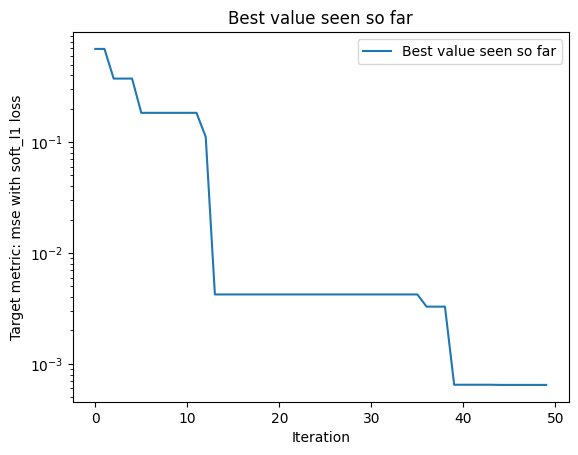
# Plot optimization results
data = ax_client.summarize()
all_metrics = optimizer.all_metrics
tracking_metrics = optimizer.all_tracking_metrics
plt.figure()
plt.plot(np.minimum.accumulate(data[all_metrics]), label="Best value seen so far")
plt.yscale("log")
plt.xlabel("Iteration")
plt.ylabel("Target metric: " + metric + " with " + loss + " loss")
plt.legend()
plt.title("Best value seen so far")
print("Best value seen so far is ", min(data[all_metrics[0]]), "at iteration ", int(data[all_metrics].idxmin()))
plt.show()
Best value seen so far is 0.00030656741921442077 at iteration 44
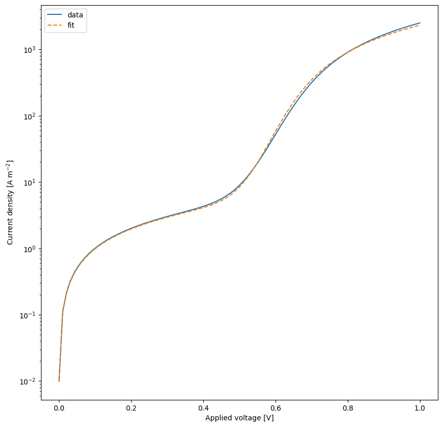
[14]:
# rerun the simulation with the best parameters
yfit = diode.run(parameters={})
plt.figure(figsize=(10,10))
plt.plot(X,y,label='data')
plt.plot(X,yfit,label='fit',linestyle='--')
plt.xscale('linear')
plt.yscale('log')
plt.xlabel('Applied voltage [V]')
plt.ylabel('Current density [A m$^{-2}$]')
plt.legend()
plt.show()
[15]:
cards = ax_client.compute_analyses(display=True)
This analysis provides an overview of the entire optimization process. It includes visualizations of the results obtained so far, insights into the parameter and metric relationships learned by the Ax model, diagnostics such as model fit, and health checks to assess the overall health of the experiment.
Result Analyses provide a high-level overview of the results of the optimization process so far with respect to the metrics specified in experiment design.
These pair of plots visualize the metric effects for each arm, with the Ax model predictions on the left and the raw observed data on the right. The predicted effects apply shrinkage for noise and adjust for non-stationarity in the data, so they are more representative of the reproducible effects that will manifest in a long-term validation experiment.
Modeled Arm Effects on diode_dark_mse_soft_l1
Modeled effects on diode_dark_mse_soft_l1. This plot visualizes predictions of the true metric changes for each arm based on Ax's model. This is the expected delta you would expect if you (re-)ran that arm. This plot helps in anticipating the outcomes and performance of arms based on the model's predictions. Note, flat predictions across arms indicate that the model predicts that there is no effect, meaning if you were to re-run the experiment, the delta you would see would be small and fall within the confidence interval indicated in the plot.
Observed Arm Effects on diode_dark_mse_soft_l1
Observed effects on diode_dark_mse_soft_l1. This plot visualizes the effects from previously-run arms on a specific metric, providing insights into their performance. This plot allows one to compare and contrast the effectiveness of different arms, highlighting which configurations have yielded the most favorable outcomes.
Summary for ax_opti
High-level summary of the `Trial`-s in this `Experiment`
| trial_index | arm_name | trial_status | generation_node | diode_dark_mse_soft_l1 | J0 | n | R_series | R_shunt | |
|---|---|---|---|---|---|---|---|---|---|
| 0 | 0 | 0_0 | COMPLETED | SOBOL | 0.363204 | -4.590296 | 1.303048 | -4.019286 | -0.213799 |
| 1 | 1 | 1_0 | COMPLETED | SOBOL | 1.479649 | -3.879895 | 1.797771 | -3.373800 | 1.969033 |
| 2 | 2 | 2_0 | COMPLETED | SOBOL | 1.833798 | -3.639844 | 1.077498 | -4.997814 | -1.839151 |
| 3 | 3 | 3_0 | COMPLETED | SOBOL | 0.835346 | -5.932277 | 1.572156 | -3.641332 | 0.095636 |
| 4 | 4 | 4_0 | COMPLETED | SOBOL | 0.951106 | -5.413541 | 1.163578 | -3.188526 | 0.883153 |
| 5 | 5 | 5_0 | COMPLETED | SOBOL | 0.398965 | -3.015635 | 1.657447 | -4.418424 | -1.174795 |
| 6 | 6 | 6_0 | COMPLETED | SOBOL | 0.970779 | -4.463083 | 1.467318 | -3.796332 | 1.009755 |
| 7 | 7 | 7_0 | COMPLETED | SOBOL | 0.457025 | -5.068021 | 1.961122 | -4.564497 | -0.800144 |
| 8 | 8 | 8_0 | COMPLETED | SOBOL | 0.561297 | -4.890716 | 1.042188 | -3.963138 | -1.307911 |
| 9 | 9 | 9_0 | COMPLETED | SOBOL | 0.743195 | -4.288617 | 1.544478 | -4.678935 | 0.501865 |
| 10 | 10 | 10_0 | COMPLETED | BOTORCH_MODULAR | 0.926657 | -5.517788 | 2.000000 | -4.251744 | -0.514306 |
| 11 | 11 | 11_0 | COMPLETED | BOTORCH_MODULAR | 0.229365 | -5.895755 | 1.303751 | -4.267829 | -0.307741 |
| 12 | 12 | 12_0 | COMPLETED | BOTORCH_MODULAR | 0.010909 | -5.941770 | 1.358370 | -4.198188 | -0.965252 |
| 13 | 13 | 13_0 | COMPLETED | BOTORCH_MODULAR | 0.918466 | -4.656674 | 1.076588 | -4.209375 | 0.188027 |
| 14 | 14 | 14_0 | COMPLETED | BOTORCH_MODULAR | 0.452122 | -6.000000 | 1.414829 | -4.122530 | -2.000000 |
| 15 | 15 | 15_0 | COMPLETED | BOTORCH_MODULAR | 0.127718 | -6.000000 | 1.492266 | -4.274292 | -1.418145 |
| 16 | 16 | 16_0 | COMPLETED | BOTORCH_MODULAR | 0.095631 | -6.000000 | 1.455720 | -4.218229 | -0.800156 |
| 17 | 17 | 17_0 | COMPLETED | BOTORCH_MODULAR | 0.034413 | -6.000000 | 1.408769 | -4.322718 | -0.953033 |
| 18 | 18 | 18_0 | COMPLETED | BOTORCH_MODULAR | 0.342559 | -4.058871 | 1.368347 | -4.237921 | -1.018658 |
| 19 | 19 | 19_0 | COMPLETED | BOTORCH_MODULAR | 0.637733 | -6.000000 | 2.000000 | -5.000000 | -1.796883 |
| 20 | 20 | 20_0 | COMPLETED | BOTORCH_MODULAR | 0.223217 | -6.000000 | 1.619335 | -4.624501 | -1.031450 |
| 21 | 21 | 21_0 | COMPLETED | BOTORCH_MODULAR | 0.006370 | -6.000000 | 1.313199 | -4.020565 | -0.913344 |
| 22 | 22 | 22_0 | COMPLETED | BOTORCH_MODULAR | 0.196107 | -5.139663 | 1.470844 | -3.000000 | -1.007741 |
| 23 | 23 | 23_0 | COMPLETED | BOTORCH_MODULAR | 0.322394 | -3.645125 | 2.000000 | -3.000000 | -1.445798 |
| 24 | 24 | 24_0 | COMPLETED | BOTORCH_MODULAR | 0.020007 | -5.308880 | 1.431816 | -4.317068 | -1.001362 |
| 25 | 25 | 25_0 | COMPLETED | BOTORCH_MODULAR | 0.080865 | -3.537193 | 2.000000 | -5.000000 | -1.283274 |
| 26 | 26 | 26_0 | COMPLETED | BOTORCH_MODULAR | 0.233986 | -6.000000 | 1.264990 | -5.000000 | -1.015149 |
| 27 | 27 | 27_0 | COMPLETED | BOTORCH_MODULAR | 0.167996 | -3.000000 | 2.000000 | -5.000000 | -0.622055 |
| 28 | 28 | 28_0 | COMPLETED | BOTORCH_MODULAR | 0.001822 | -5.619787 | 1.343401 | -3.913529 | -1.003001 |
| 29 | 29 | 29_0 | COMPLETED | BOTORCH_MODULAR | 0.132930 | -6.000000 | 1.112306 | -3.000000 | -0.982364 |
| 30 | 30 | 30_0 | COMPLETED | BOTORCH_MODULAR | 0.030243 | -3.000000 | 2.000000 | -4.100186 | -1.058706 |
| 31 | 31 | 31_0 | COMPLETED | BOTORCH_MODULAR | 0.486667 | -3.000000 | 2.000000 | -4.152638 | -2.000000 |
| 32 | 32 | 32_0 | COMPLETED | BOTORCH_MODULAR | 0.003085 | -3.659785 | 1.898152 | -4.242615 | -1.005080 |
| 33 | 33 | 33_0 | COMPLETED | BOTORCH_MODULAR | 0.240925 | -3.000000 | 1.891218 | -3.000328 | -0.425735 |
| 34 | 34 | 34_0 | COMPLETED | BOTORCH_MODULAR | 0.004959 | -3.447249 | 2.000000 | -4.277401 | -1.010755 |
| 35 | 35 | 35_0 | COMPLETED | BOTORCH_MODULAR | 0.003070 | -4.379335 | 1.686571 | -4.199914 | -1.030470 |
| 36 | 36 | 36_0 | COMPLETED | BOTORCH_MODULAR | 0.030384 | -4.128059 | 1.815926 | -4.337234 | -1.213153 |
| 37 | 37 | 37_0 | COMPLETED | BOTORCH_MODULAR | 0.006142 | -3.969876 | 1.741910 | -3.977862 | -0.885914 |
| 38 | 38 | 38_0 | COMPLETED | BOTORCH_MODULAR | 0.000423 | -4.844851 | 1.547697 | -4.045480 | -0.981934 |
| 39 | 39 | 39_0 | COMPLETED | BOTORCH_MODULAR | 0.002257 | -6.000000 | 1.276506 | -3.882556 | -1.027823 |
| 40 | 40 | 40_0 | COMPLETED | BOTORCH_MODULAR | 0.011287 | -4.126967 | 1.730261 | -4.312465 | -0.898845 |
| 41 | 41 | 41_0 | COMPLETED | BOTORCH_MODULAR | 0.004380 | -4.250311 | 1.680157 | -3.899559 | -1.023129 |
| 42 | 42 | 42_0 | COMPLETED | BOTORCH_MODULAR | 0.001960 | -4.478207 | 1.624959 | -4.045852 | -0.929756 |
| 43 | 43 | 43_0 | COMPLETED | BOTORCH_MODULAR | 0.004135 | -3.526035 | 1.890770 | -4.050247 | -0.933335 |
| 44 | 44 | 44_0 | COMPLETED | BOTORCH_MODULAR | 0.000307 | -5.442161 | 1.413871 | -4.004229 | -1.001955 |
| 45 | 45 | 45_0 | COMPLETED | BOTORCH_MODULAR | 0.015124 | -6.000000 | 1.236531 | -3.887316 | -0.914294 |
| 46 | 46 | 46_0 | COMPLETED | BOTORCH_MODULAR | 0.001210 | -3.968483 | 1.784712 | -4.075420 | -0.987827 |
| 47 | 47 | 47_0 | COMPLETED | BOTORCH_MODULAR | 0.000889 | -5.766214 | 1.345592 | -4.006581 | -1.018440 |
| 48 | 48 | 48_0 | COMPLETED | BOTORCH_MODULAR | 0.002501 | -4.660638 | 1.586361 | -4.056858 | -1.067384 |
| 49 | 49 | 49_0 | COMPLETED | BOTORCH_MODULAR | 0.000436 | -5.123975 | 1.461855 | -3.976050 | -1.020017 |
Insight Analyses display information to help understand the underlying experiment i.e parameter and metric relationships learned by the Ax model.Use this information to better understand your experiment space and users.
The top surfaces analysis displays three analyses in one. First, it shows parameter sensitivities, which shows the sensitivity of the metrics in the experiment to the most important parameters. Subsetting to only the most important parameters, it then shows slice plots and contour plots for each metric in the experiment, displaying the relationship between the metric and the most important parameters.
Sensitivity Analysis for diode_dark_mse_so...
Understand how each parameter affects diode_dark_mse_so... according to a second-order sensitivity analysis.
These plots show the relationship between a metric and a parameter. They show the predicted values of the metric on the y-axis as a function of the parameter on the x-axis while keeping all other parameters fixed at their status_quo value (or mean value if status_quo is unavailable).
diode_dark_mse_soft_l1 vs. R_shunt
The slice plot provides a one-dimensional view of predicted outcomes for diode_dark_mse_soft_l1 as a function of a single parameter, while keeping all other parameters fixed at their status_quo value (or mean value if status_quo is unavailable). This visualization helps in understanding the sensitivity and impact of changes in the selected parameter on the predicted metric outcomes.
diode_dark_mse_soft_l1 vs. n
The slice plot provides a one-dimensional view of predicted outcomes for diode_dark_mse_soft_l1 as a function of a single parameter, while keeping all other parameters fixed at their status_quo value (or mean value if status_quo is unavailable). This visualization helps in understanding the sensitivity and impact of changes in the selected parameter on the predicted metric outcomes.
These plots show the relationship between a metric and two parameters. They show the predicted values of the metric (indicated by color) as a function of the two parameters on the x- and y-axes while keeping all other parameters fixed at their status_quo value (or mean value if status_quo is unavailable).
diode_dark_mse_soft_l1 vs. J0, n
The contour plot visualizes the predicted outcomes for diode_dark_mse_soft_l1 across a two-dimensional parameter space, with other parameters held fixed at their status_quo value (or mean value if status_quo is unavailable). This plot helps in identifying regions of optimal performance and understanding how changes in the selected parameters influence the predicted outcomes. Contour lines represent levels of constant predicted values, providing insights into the gradient and potential optima within the parameter space.
Diagnostic Analyses provide information about the optimization process and the quality of the model fit. You can use this information to understand if the experimental design should be adjusted to improve optimization quality.
Cross-validation plots display the model fit for each metric in the experiment. The model is trained on a subset of the data and then predicts the outcome for the remaining subset. The plots show the predicted outcome for the validation set on the y-axis against its actual value on the x-axis. Points that align closely with the dotted diagonal line indicate a strong model fit, signifying accurate predictions. Additionally, the plots include confidence intervals that provide insight into the noise in observations and the uncertainty in model predictions.
NOTE: A horizontal, flat line of predictions indicates that the model has not picked up on sufficient signal in the data, and instead is just predicting the mean.
Cross Validation for diode_dark_mse_soft_l1
The cross-validation plot displays the model fit for each metric in the experiment. It employs a leave-one-out approach, where the model is trained on all data except one sample, which is used for validation. The plot shows the predicted outcome for the validation set on the y-axis against its actual value on the x-axis. Points that align closely with the dotted diagonal line indicate a strong model fit, signifying accurate predictions. Additionally, the plot includes 95% confidence intervals that provide insight into the noise in observations and the uncertainty in model predictions. A horizontal, flat line of predictions indicates that the model has not picked up on sufficient signal in the data, and instead is just predicting the mean.
Moving on to the scipy optimizer
[16]:
params_scipy = deepcopy(diode.params) # make copies of the parameters
# change the values of params scipy by a random value between the bounds
for param in params_scipy:
param.value = np.random.uniform(param.bounds[0], param.bounds[1])
print(f'param: {param.name}, value: {param.value}, bounds: {param.bounds}')
# Create a new agent with the new parameters
# this is needed as the scipy optimizer uses the parameters values as the initial guess for the optimization
diode2 = deepcopy(diode) # make a copy of the agent
diode2.params = params_scipy # set the new parameters
from optimpv.optimizers.scipyOpti.scipyOptimizer import ScipyOptimizer
scipyOpti = ScipyOptimizer(params=params_scipy, agents=diode2, method='dogbox', options={'max_nfev': 10000}, name='scipy_opti', parallel_agents=True, max_parallelism=os.cpu_count()-1, verbose_logging=True)
param: J0, value: 0.0005223391156617449, bounds: [1e-06, 0.001]
param: n, value: 1.4324097248686063, bounds: [1, 2]
param: R_series, value: 0.0007100445020787827, bounds: [1e-05, 0.001]
param: R_shunt, value: 13.229354725232643, bounds: [0.01, 100.0]
[17]:
scipyOpti.optimize_least_squares() # run the optimization with scipy least squares
Starting optimization using dogbox method
Optimization completed with status: `gtol` termination condition is satisfied.
Final objective value: [2.91914009e-05]
[17]:
message: `gtol` termination condition is satisfied.
success: True
status: 1
fun: [ 2.919e-05]
x: [-4.794e+00 1.548e+00 -4.016e+00 -9.972e-01]
cost: 4.260689442007881e-10
jac: [[ 3.425e-04 -2.299e-04 -6.826e-05 -1.654e-05]]
grad: [ 9.999e-09 -6.712e-09 -1.993e-09 -4.828e-10]
optimality: 9.998779724557937e-09
active_mask: [0 0 0 0]
nfev: 2991
njev: 2933
[18]:
# get the best parameters and update the params list in the optimizer and the agent
diode2.params = scipyOpti.params # update the params list in the agent with the best parameters.append
# print the best parameters
print('Best parameters:')
for p,po in zip(scipyOpti.params, params_orig):
if p.axis_type == 'log':
print(p.name, 'fitted value:', '{:.2e}'.format(p.value), 'original value:', '{:.2e}'.format(po.value))
else:
print(p.name, 'fitted value:', p.value, 'original value:', po.value)
Best parameters:
J0 fitted value: 1.61e-05 original value: 1.00e-05
n fitted value: 1.5481726513230254 original value: 1.5
R_series fitted value: 9.64e-05 original value: 1.00e-04
R_shunt fitted value: 1.01e-01 original value: 1.00e-01
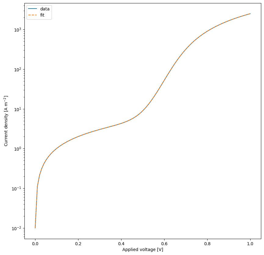
[19]:
# rerun the simulation with the best parameters
yfit = diode2.run(parameters={})
plt.figure(figsize=(10,10))
plt.plot(X,y,label='data')
plt.plot(X,yfit,label='fit',linestyle='--')
plt.xscale('linear')
plt.yscale('log')
plt.xlabel('Applied voltage [V]')
plt.ylabel('Current density [A m$^{-2}$]')
plt.legend()
plt.show()
Define the parameters for the simulation for light JV
Now we run only the scipy optimization to fit the light JV-curve.
[20]:
##############################################################################################
# Define the parameters to be fitted
params = []
J0 = FitParam(name = 'J0', value = 1e-6, bounds = [1e-7,1e-4], log_scale = True, rescale = False, value_type = 'float', type='range', display_name=r'$J_0$', unit='A m$^{-2}$', axis_type = 'log',force_log=True)
params.append(J0)
n = FitParam(name = 'n', value = 1.5, bounds = [1,2], log_scale = False, value_type = 'float', type='range', display_name=r'$n$', unit='', axis_type = 'linear')
params.append(n)
R_series = FitParam(name = 'R_series', value = 1e-4, bounds = [1e-5,1e-3], log_scale = True, rescale = False, value_type = 'float', type='range', display_name=r'$R_{\text{series}}$', unit=r'$\Omega$ m$^2$', axis_type = 'log',force_log=True)
params.append(R_series)
R_shunt = FitParam(name = 'R_shunt', value = 1e-1, bounds = [1e-2,1e2], log_scale = True, rescale = False, value_type = 'float', type='range', display_name=r'$R_{\text{shunt}}$', unit=r'$\Omega$ m$^2$', axis_type = 'log',force_log=True)
params.append(R_shunt)
Jph = FitParam(name = 'Jph', value = 200, bounds = [150,250], log_scale = False, rescale = False, value_type = 'float', type='range', display_name=r'$J_{\text{ph}}$', unit='A m$^{-2}$', axis_type = 'linear')
params.append(Jph)
# original values
params_orig_light = copy.deepcopy(params)
num_free_params = len([p for p in params if p.type != 'fixed'])
[21]:
# Create JV to fit
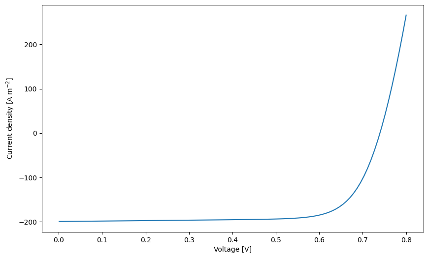
X_light = np.linspace(0.001,0.8,100)
y_light = NonIdealDiode_light(X_light, J0.value, n.value, R_series.value, R_shunt.value, Jph.value)
plt.figure(figsize=(10,6))
plt.plot(X_light,y_light)
plt.xlabel('Voltage [V]')
plt.ylabel('Current density [A m$^{-2}$]')
[21]:
Text(0, 0.5, 'Current density [A m$^{-2}$]')
Run the optimization
[22]:
# Define the agents
metric = 'nrmse' # can be 'nrmse', 'mse', 'mae'
loss = 'linear' # can be 'linear', 'huber', 'soft_l1'
exp_format = 'light' # can be 'dark', 'light' depending on the type of data you have
use_pvlib = False # if True, use pvlib to calculate the diode model if not use the implementation in DiodeModel.py
diode_light = DiodeAgent(params, X_light, y_light, metric = metric, loss = loss, minimize=True,exp_format=exp_format,use_pvlib=False)
[23]:
params_scipy_light = deepcopy(diode_light.params) # make copies of the parameters
# change the values of params scipy by a random value between the bounds
for param in params_scipy_light:
param.value = np.random.uniform(param.bounds[0], param.bounds[1])
print(f'param: {param.name}, value: {param.value}, bounds: {param.bounds}')
# Create a new agent with the new parameters
# this is needed as the scipy optimizer uses the parameters values as the initial guess for the optimization
diode2_light = deepcopy(diode_light) # make a copy of the agent
diode2_light.params = params_scipy_light # set the new parameters
from optimpv.optimizers.scipyOpti.scipyOptimizer import ScipyOptimizer
scipyOpti_light = ScipyOptimizer(params=params_scipy_light, agents=diode2_light, method='L-BFGS-B', options={'maxiter':int(1e5),'ftol':1e-13,'xtol':1e-10}, name='scipy_opti', parallel_agents=True, max_parallelism=os.cpu_count()-1, verbose_logging=True)
param: J0, value: 7.238779618275176e-05, bounds: [1e-07, 0.0001]
param: n, value: 1.7114094391492194, bounds: [1, 2]
param: R_series, value: 0.0005150939424732479, bounds: [1e-05, 0.001]
param: R_shunt, value: 41.89968279615289, bounds: [0.01, 100.0]
param: Jph, value: 205.27983292254527, bounds: [150, 250]
[24]:
scipyOpti_light.optimize() # run the optimization with scipy
Starting optimization using L-BFGS-B method
Optimization completed with status: CONVERGENCE: RELATIVE REDUCTION OF F <= FACTR*EPSMCH
Final objective value: 0.00282924221851808
[24]:
message: CONVERGENCE: RELATIVE REDUCTION OF F <= FACTR*EPSMCH
success: True
status: 0
fun: 0.00282924221851808
x: [-5.276e+00 1.642e+00 -4.053e+00 1.473e+00 1.971e+02]
nit: 72
jac: [ 5.025e-06 -2.424e-05 -3.701e-06 2.155e-05 -3.440e-07]
nfev: 672
njev: 112
hess_inv: <5x5 LbfgsInvHessProduct with dtype=float64>
[25]:
# get the best parameters and update the params list in the optimizer and the agent
diode2_light.params = scipyOpti_light.params # update the params list in the agent with the best parameters.append
# print the best parameters
print('Best parameters:')
for p,po in zip(scipyOpti_light.params, params_orig_light):
if p.axis_type == 'log':
print(p.name, 'fitted value:', '{:.2e}'.format(p.value), 'original value:', '{:.2e}'.format(po.value))
else:
print(p.name, 'fitted value:', p.value, 'original value:', po.value)
Best parameters:
J0 fitted value: 5.30e-06 original value: 1.00e-06
n fitted value: 1.6418703491148807 original value: 1.5
R_series fitted value: 8.85e-05 original value: 1.00e-04
R_shunt fitted value: 2.97e+01 original value: 1.00e-01
Jph fitted value: 197.0905300005406 original value: 200
[26]:
# rerun the simulation with the best parameters
yfit_light = diode2_light.run(parameters={})
plt.figure(figsize=(10,10))
plt.plot(X_light,y_light,label='data')
plt.plot(X_light,yfit_light,label='fit',linestyle='--')
plt.xscale('linear')
# plt.yscale('log')
plt.xlabel('Applied voltage [V]')
plt.ylabel('Current density [A m$^{-2}$]')
plt.legend()
plt.show()
