Approximate Posterior Probability Distributions
This notebook is a demonstration of how to fit light-intensity dependent JV curves with drift-diffusion models using the SIMsalabim package.
It also shows how to compute and visualize approximate posterior probability distributions of the fitted parameters using the ApproximatePosterior class from the optimpv package.
The ApproximatePosterior builds a surrogate model using BoTorch Gaussian Processes to learn the log-likelihood landscape. It can then be used to quickly evaluate and visualize the posterior distributions of the fitted parameters without the need of sampling the DD model directly (which can be computationally expensive) or without building a complicated surrogate model to replace the DD model.
[ ]:
# Import necessary libraries
import warnings, os, sys, shutil
# remove warnings from the output
os.environ["PYTHONWARNINGS"] = "ignore"
warnings.filterwarnings(action='ignore', category=FutureWarning)
warnings.filterwarnings(action='ignore', category=UserWarning)
os.environ['PYTORCH_CUDA_ALLOC_CONF'] = 'expandable_segments:True'
import pandas as pd
import matplotlib.pyplot as plt
import numpy as np
from numpy.random import default_rng
import torch, copy, uuid
import pySIMsalabim as sim
from pySIMsalabim.experiments.JV_steady_state import *
import ax, logging
from ax.utils.notebook.plotting import init_notebook_plotting, render
init_notebook_plotting() # for Jupyter notebooks

try:
    from optimpv import *
    from optimpv.optimizers.axBOtorch.axUtils import *
except Exception as e:
    sys.path.append('../') # add the path to the optimpv module
    from optimpv import *
    from optimpv.optimizers.axBOtorch.axUtils import *
[INFO 01-20 10:12:44] ax.utils.notebook.plotting: Injecting Plotly library into cell. Do not overwrite or delete cell.
[INFO 01-20 10:12:44] ax.utils.notebook.plotting: Please see
    (https://ax.dev/tutorials/visualizations.html#Fix-for-plots-that-are-not-rendering)
    if visualizations are not rendering.
Define the parameters for the simulation
[2]:
params = [] # list of parameters to be optimized

mup = FitParam(name = 'l2.mu_p', value = 5e-9, bounds = [5e-10,1e-6], log_scale = True, value_type = 'float', fscale = None, rescale = False, display_name=r'$\mu_p$', unit=r'm$^2$ V$^{-1}$s$^{-1}$', axis_type = 'log', force_log = True)
params.append(mup)

mun = FitParam(name = 'l2.mu_n', value = 3e-7, bounds = [5e-10,1e-6], log_scale = True, value_type = 'float', fscale = None, rescale = False, display_name=r'$\mu_n$', unit='m$^2$ V$^{-1}$s$^{-1}$', axis_type = 'log', force_log = True)
params.append(mun)

bulk_tr = FitParam(name = 'l2.N_t_bulk', value = 1e20, bounds = [1e19,1e22], log_scale = True, value_type = 'float', fscale = None, rescale = False,  display_name=r'$N_{T}$', unit=r'm$^{-3}$', axis_type = 'log', force_log = True)
params.append(bulk_tr)

preLangevin = FitParam(name = 'l2.preLangevin', value = 1e-2, bounds = [0.005,1], log_scale = True, value_type = 'float', fscale = None, rescale = False, display_name=r'$\gamma_{pre}$', unit=r'-', axis_type = 'log', force_log = True)
params.append(preLangevin)

R_series = FitParam(name = 'R_series', value = 1e-4, bounds = [1e-5,1e-1], log_scale = True, value_type = 'float', fscale = None, rescale = False,  display_name=r'$R_{series}$', unit=r'$\Omega$ m$^2$', axis_type = 'log', force_log = True)
params.append(R_series)

R_shunt = FitParam(name = 'R_shunt', value = 1e1, bounds = [1e-2,1e2], log_scale = True, value_type = 'float', fscale = None, rescale = False,  display_name=r'$R_{shunt}$', unit=r'$\Omega$ m$^2$', axis_type = 'log', force_log = True)
params.append(R_shunt)


# save the original parameters for later
params_orig = copy.deepcopy(params)
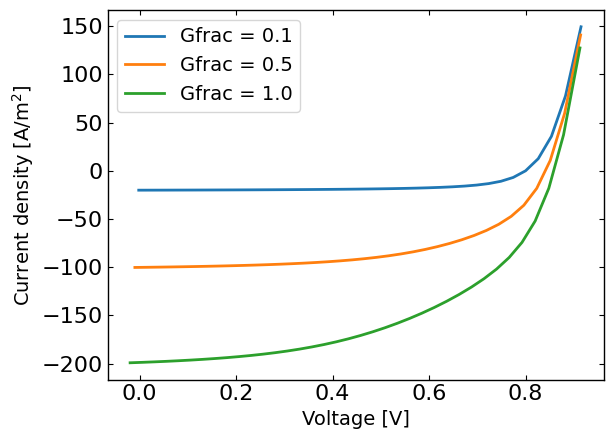
Generate some fake data
Here we generate some fake data to fit. The data is generated using the same model as the one used for the fitting, so it is a good test of the fitting procedure. For more information on how to run SIMsalabim from python see the pySIMsalabim package.
[3]:
# Set the session path for the simulation and the input files
session_path = os.path.join(os.path.join(os.path.abspath('../'),'SIMsalabim','SimSS'))
input_path = os.path.join(os.path.join(os.path.join(os.path.abspath('../'),'Data','simsalabim_test_inputs','fakeOPV')))
simulation_setup_filename = 'simulation_setup_fakeOPV.txt'
simulation_setup = os.path.join(session_path, simulation_setup_filename)
# path to the layer files defined in the simulation_setup file
l1 = 'ZnO.txt'
l2 = 'ActiveLayer.txt'
l3 = 'BM_HTL.txt'
l1 = os.path.join(input_path, l1)
l2 = os.path.join(input_path, l2)
l3 = os.path.join(input_path, l3)
# copy this files to session_path
force_copy = True
if not os.path.exists(session_path):
os.makedirs(session_path)
for file in [l1,l2,l3,simulation_setup_filename]:
file = os.path.join(input_path, os.path.basename(file))
if force_copy or not os.path.exists(os.path.join(session_path, os.path.basename(file))):
shutil.copyfile(file, os.path.join(session_path, os.path.basename(file)))
else:
print('File already exists: ',file)
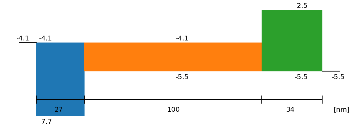
# Show the device structure
fig = sim.plot_band_diagram(simulation_setup, session_path)
# reset simss
# Set the JV parameters
Gfracs = [0.1,0.5,1.0] # Fractions of the generation rate to simulate (None if you want only one light intensity as define in the simulation_setup file)
UUID = str(uuid.uuid4()) # random UUID to avoid overwriting files
cmd_pars = [] # see pySIMsalabim documentation for the command line parameters
# Add the parameters to the command line arguments
for param in params:
cmd_pars.append({'par':param.name, 'val':str(param.value)})
# Run the JV simulation
ret, mess = run_SS_JV(simulation_setup, session_path, JV_file_name = 'JV.dat', G_fracs = Gfracs, parallel = True, max_jobs = 3, UUID=UUID, cmd_pars=cmd_pars)
# save data for fitting
X,y = [],[]
X_orig,y_orig = [],[]
if Gfracs is None:
data = pd.read_csv(os.path.join(session_path, 'JV_'+UUID+'.dat'), sep=r'\s+') # Load the data
Vext = np.asarray(data['Vext'].values)
Jext = np.asarray(data['Jext'].values)
G = np.ones_like(Vext)
rng = default_rng()#
noise = rng.standard_normal(Jext.shape) * 0.01 * Jext
Jext = Jext + noise
X = Vext
y = Jext
plt.figure()
plt.plot(X,y)
plt.show()
else:
for Gfrac in Gfracs:
data = pd.read_csv(os.path.join(session_path, 'JV_Gfrac_'+str(Gfrac)+'_'+UUID+'.dat'), sep=r'\s+') # Load the data
Vext = np.asarray(data['Vext'].values)
Jext = np.asarray(data['Jext'].values)
G = np.ones_like(Vext)*Gfrac
rng = default_rng()#
noise = 0 #rng.standard_normal(Jext.shape) * 0.005 * Jext
if len(X) == 0:
X = np.vstack((Vext,G)).T
y = Jext + noise
y_orig = Jext
else:
X = np.vstack((X,np.vstack((Vext,G)).T))
y = np.hstack((y,Jext+ noise))
y_orig = np.hstack((y_orig,Jext))
# remove all the current where Jext is higher than a given value
X = X[y<200]
X_orig = copy.deepcopy(X)
y_orig = y_orig[y<200]
y = y[y<200]
plt.figure()
for Gfrac in Gfracs:
plt.plot(X[X[:,1]==Gfrac,0],y[X[:,1]==Gfrac],label='Gfrac = '+str(Gfrac))
plt.xlabel('Voltage [V]')
plt.ylabel('Current density [A/m$^2$]')
plt.legend()
plt.show()
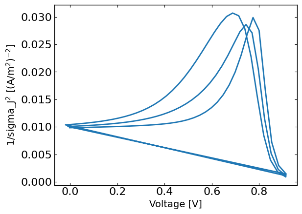
# The following calculates sigma using a similar approach as in Eunchi Kim et al. DOI: 10.1002/solr.202500648
# calculate the sigma for the experimental data
std_phi = 0.05 # 5% error on light intensity
std_vol = 0.01 # 10 mV error on voltage
# reshape y such that each Gfrac is a column
y_reshaped = y.reshape((len(Gfracs), int(len(y)/len(Gfracs)))) # normalize to 10 A/m2
# get dy/dGfrac
dJ_dphi = np.gradient(y_reshaped,Gfracs,axis=0,edge_order=2)
dJ_dV = np.gradient(y_reshaped,X[:,0][X[:,1]==Gfracs[0]],axis=1,edge_order=2)
phi_term = (std_phi * dJ_dphi)**2
vol_term = (std_vol * dJ_dV)**2
phi_term = phi_term.flatten()
vol_term = vol_term.flatten()
sigma_J = np.sqrt((std_phi*dJ_dphi)**2 + (std_vol*dJ_dV)**2)
sigma_J = sigma_J.flatten() # convert to absolute error
plt.figure()
plt.plot(X[:,0],1/sigma_J**2)
plt.xlabel('Voltage [V]')
plt.ylabel('1/sigma_J$^2$ [(A/m$^2$)$^{-2}$]')
plt.show()
Define the JVAgent
[ ]:
# Define the Agent and the target metric/loss function
from optimpv.models.DDfits.JVAgent import JVAgent
metric = 'nrmse' # can be 'nrmse', 'mse', 'mae'
loss = 'linear' # can be 'linear', 'huber', 'soft_l1'

# Here we are doing the optimization on nrmse as it seems to work well in general for JV fits
# but we are tracking the LLH with a weighting corresponding to sigma_J as we need it later for the approximate posterior
tracking_metrics = 'LLH' # can be 'nrmse', 'mse', 'mae', 'LLH'
tracking_loss = 'linear' # can be 'linear', 'huber', 'soft_l1'
tracking_weight = 1/sigma_J**2
tracking_X = X
tracking_y = y
tracking_exp_format = 'JV'
jv = JVAgent(params, X, y, session_path, simulation_setup, parallel = True, max_jobs = 3, metric = metric, loss = loss,tracking_metric = tracking_metrics, tracking_loss = tracking_loss,tracking_weight = tracking_weight,tracking_X=tracking_X, tracking_y=tracking_y, tracking_exp_format=tracking_exp_format)
Run the optimization
[ ]:
from optimpv.optimizers.axBOtorch.axBOtorchOptimizer import axBOtorchOptimizer
from optimpv.optimizers.axBOtorch.axUtils import get_VMLC_default_model_kwargs_list
import ray

@ray.remote
def run_optimization_chain(chain_id, params, jv, num_free_params):
    """
    Run a single optimization chain with Ray.
    """
    print(f"Starting optimization chain {chain_id}")
    optimizer = axBOtorchOptimizer(
        params=params,
        agents=jv,
        models=['SOBOL', 'BOTORCH_MODULAR'],
        n_batches=[5, 100],
        batch_size=[5, 2],
        ax_client=None,
        max_parallelism=-1,
        model_kwargs_list=get_VMLC_default_model_kwargs_list(num_free_params=num_free_params),
        model_gen_kwargs_list=None,
        name=f'ax_opti_chain_{chain_id}',
        parallel=True,
        verbose_logging=False,
    )
    optimizer.optimize_turbo()
    return optimizer.ax_client.summarize()

# Run optimization chains with Ray
n_chains = 10
if not ray.is_initialized():
    ray.init(ignore_reinit_error=True, num_cpus=n_chains)

num_free_params = len([p for p in params if getattr(p, "type", "free") != "fixed"])
futures = [
    run_optimization_chain.remote(i + 1, params, jv, num_free_params)
    for i in range(n_chains)
]
results = ray.get(futures)

data_main = pd.concat(results, ignore_index=True)
print("All chains completed.")
2026-01-20 10:12:49,097 INFO worker.py:2014 -- Started a local Ray instance. View the dashboard at http://127.0.0.1:8265
(run_optimization_chain pid=209810) Starting optimization chain 8
(run_optimization_chain pid=209804) [WARNING 01-20 10:13:55] ax.api.client: Metric IMetric('JV_JV_LLH_linear') not found in optimization config, added as tracking metric.
(run_optimization_chain pid=209805) [WARNING 01-20 10:14:13] ax.api.client: Metric IMetric('JV_JV_LLH_linear') not found in optimization config, added as tracking metric. [repeated 2x across cluster] (Ray deduplicates logs by default. Set RAY_DEDUP_LOGS=0 to disable log deduplication, or see https://docs.ray.io/en/master/ray-observability/user-guides/configure-logging.html#log-deduplication for more options.)
(run_optimization_chain pid=209809) [WARNING 01-20 10:14:31] ax.api.client: Metric IMetric('JV_JV_LLH_linear') not found in optimization config, added as tracking metric. [repeated 3x across cluster]
(run_optimization_chain pid=209806) [WARNING 01-20 10:14:38] ax.api.client: Metric IMetric('JV_JV_LLH_linear') not found in optimization config, added as tracking metric.
(run_optimization_chain pid=209811) [ERROR 01-20 10:14:42] optimpv.axBOtorchOptimizer: Error in Turbo batch 102: All attempts to fit the model have failed.
(run_optimization_chain pid=209811) [ERROR 01-20 10:14:42] optimpv.axBOtorchOptimizer: We are stopping the optimization process
(run_optimization_chain pid=209811) [WARNING 01-20 10:14:42] ax.api.client: Metric IMetric('JV_JV_LLH_linear') not found in optimization config, added as tracking metric.
(run_optimization_chain pid=209802) [WARNING 01-20 10:14:49] ax.api.client: Metric IMetric('JV_JV_LLH_linear') not found in optimization config, added as tracking metric.
(run_optimization_chain pid=209803) [WARNING 01-20 10:14:52] ax.api.client: Metric IMetric('JV_JV_LLH_linear') not found in optimization config, added as tracking metric.
All chains completed.
Calculate and visualize the approximate posterior distributions
Here we have multiple options to calculate and visualize the approximate posterior distributions:
Calculate slice plots of the approximated posterior distributions, where all the parameters are fixed to their best-fit values except for one or two parameters which are varied over a range of values. This gives a 1D or 2D slice of the posterior distribution.
Calculate and visualize the marginal posterior distributions of each parameter by integrating over the other parameters this integration is done by creating a grid of points in the parameter space and evaluating the approximate posterior at each point. Then the marginal distributions are obtained by summing over the other parameters. Note that this can be computationally expensive for high-dimensional parameter spaces, so you have to limit the number of grid points used for the integration.
Use MCMC and NUTS sampling to sample from the approximate posterior distribution using the surrogate model. While this is implementend, it does not seem to work very well yet and is still experimental. The accuracy of the surrogate model is crucial for this to work well which is difficult to achieve without a lot of training data. The edge of the parameter space is particularly difficult to model accurately which can lead to biased results.
[6]:
from optimpv.posterior.approx_posterior import *
names = [param.name for param in params]
outcome_name = 'JV_JV_LLH_linear'

approx_post = ApproximatePosterior(params, data_main,sigma_J, outcome_name,loss='linear',max_size_cv=10,device='cpu') # here we use cpu to avoid cuda memory issues when doing the grid calculations
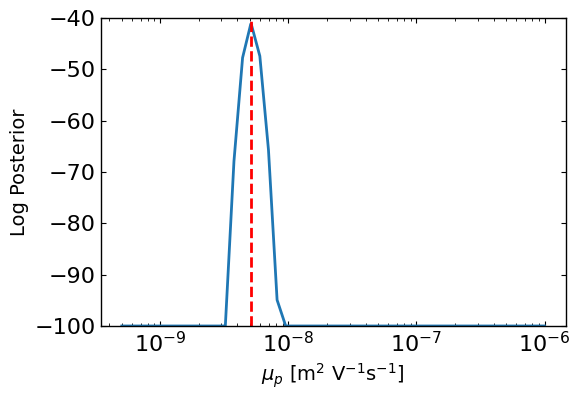
First the slice posterior plots
[7]:
ax1 = approx_post.plot_1d_posteriors_slice(params[0].name,Nres=50,vmin=-100,show_best_param=True)
[8]:
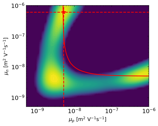
ax2 = approx_post.plot_2d_posteriors_slice(params[0].name,params[1].name,Nres=50,vmin=-300)

# here we are simulating a mostly symmetric case where mu_p and mu_n best values can be reversed.
# So we can plot the contour where mu_eff is constant, and we see well that the posterior follows this line and that the best parameter values are symmetric.
mu_target = params_orig[0].value * params_orig[1].value / (params_orig[0].value + params_orig[1].value)
mu_n_vals = np.logspace(np.log10(params[1].bounds[0]), np.log10(params[1].bounds[1]), 100)
mu_p_vals = (mu_target * mu_n_vals) / ((mu_n_vals - mu_target))

# Define range for x and y
X_, Y_ = np.meshgrid(np.linspace(params[0].bounds[0], params[0].bounds[1], 400),np.linspace(params[1].bounds[0], params[1].bounds[1], 400))
C = params_orig[0].value * params_orig[1].value / (params_orig[0].value + params_orig[1].value)
Z = (X_ * Y_) / (X_ + Y_)
Z = np.ma.masked_invalid(Z)
ax2.contour(X_, Y_, Z, levels=[C], colors='r')
[8]:
<matplotlib.contour.QuadContourSet at 0x7c19dc6a1590>
[9]:
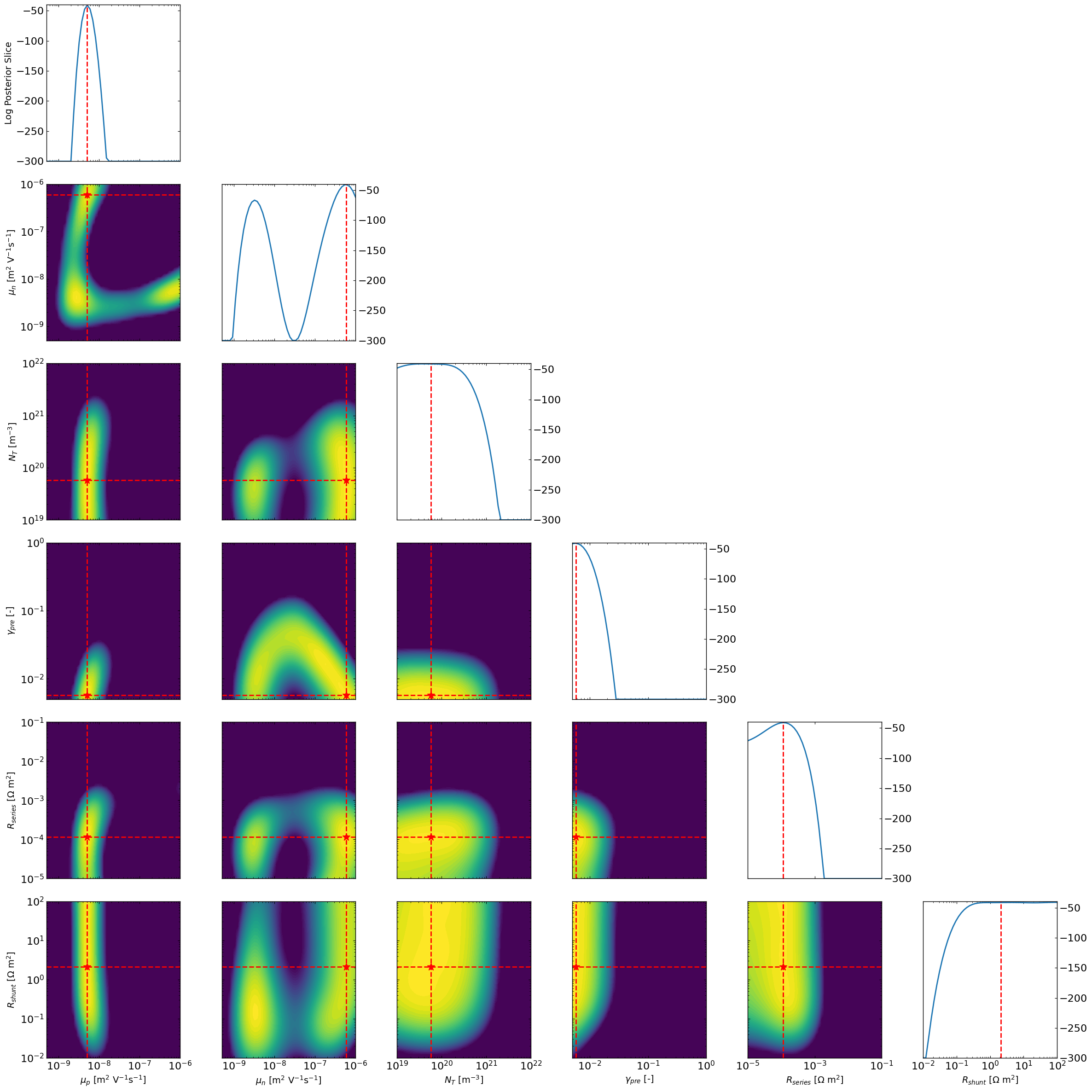
# All combinations of slice plots
ax3 = approx_post.plot_all_posteriors_slices(Nres = 50, slice_param=None,slice_nat_scale=False,vmin=-300)
Now we can look at the marginal posterior distributions using a grid approach
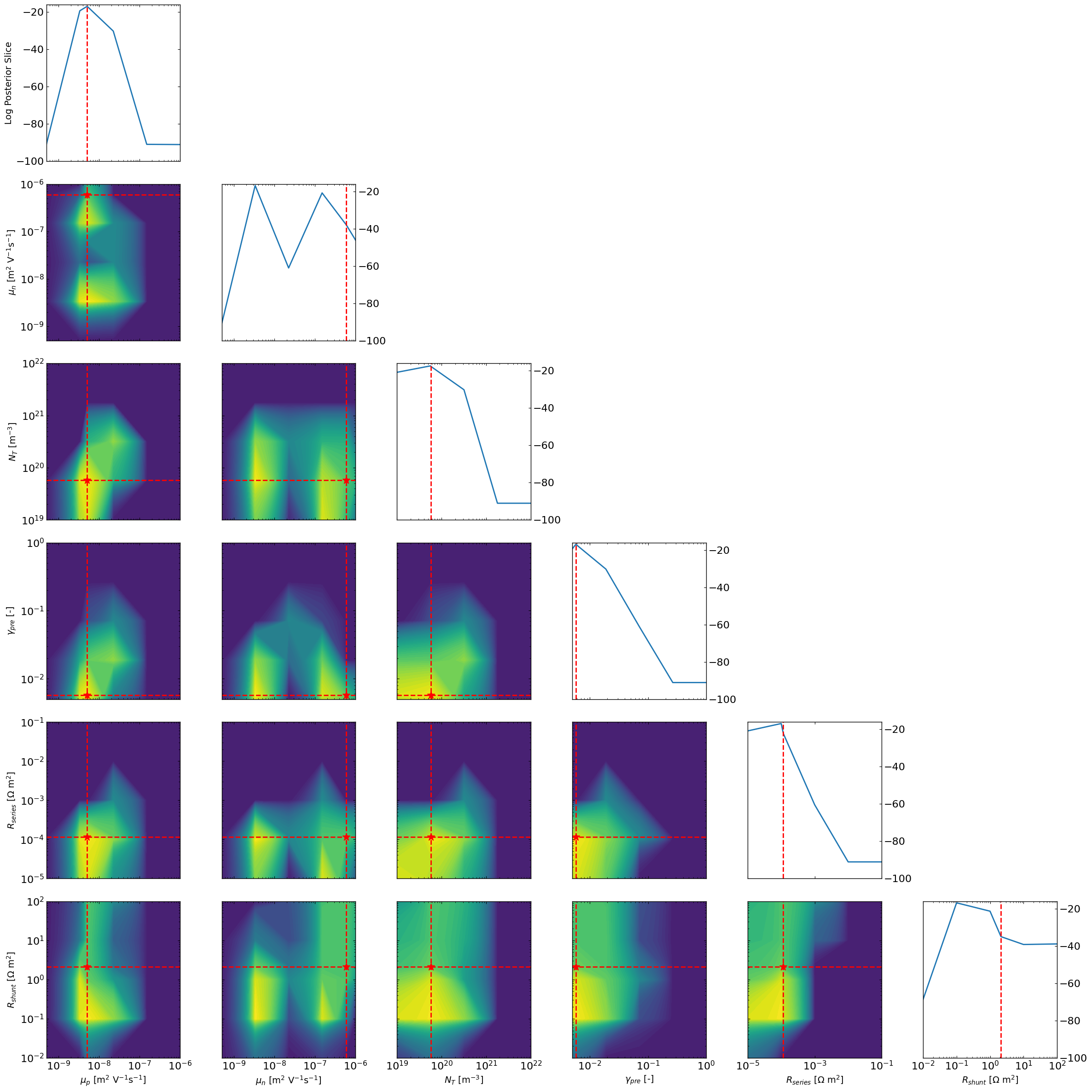
[10]:
ax4 = approx_post.plot_all_posteriors_marginal_grid(Nres=5,vmin=-100,)
Now we can try MCMC with NUTS sampling to sample from the approximate posterior distributions
The accuracy of this method is really unclear, the mcmc tend to get stuck and over-sample the edges for some of the parameters especially when the posterior is expected to be mostly flat. Maybe this can be improved with a better surrogate or a different sampling method.
[11]:
approx_post2 = ApproximatePosterior(params, data_main,sigma_J, outcome_name,loss='linear',max_size_cv=10,device='cpu')
mcmc, samples, az_data = approx_post2.calculate_posteriors_mcmc_nuts(num_samples=1000, warmup_steps=300, num_chains=5,initialize_with_best=False)
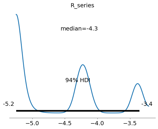
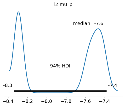
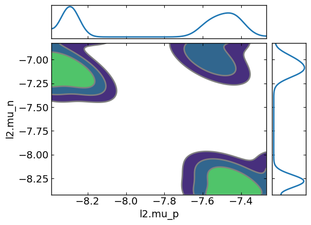
[12]:
import arviz as az
# Note that the plots from the mcmc are on scaled data
ax5 = az.plot_posterior(az_data, point_estimate='median',var_names=[params[4].name])
ax6 = az.plot_posterior(az_data, point_estimate='median',var_names=[params[0].name])
ax7 = az.plot_pair(az_data, kind='kde', marginals=True,var_names=[params[0].name,params[1].name])
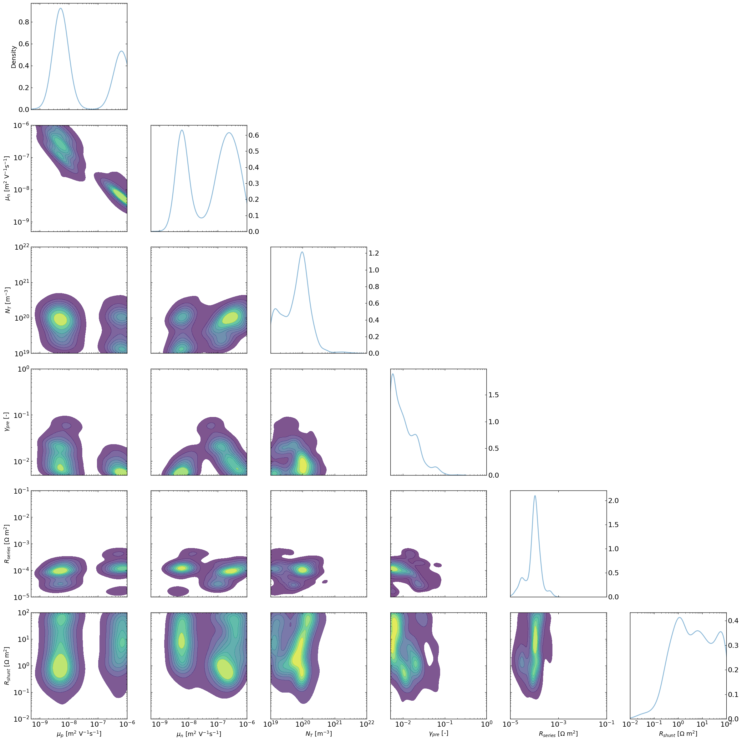
The “lazy” posterior
The following implementation has NO mathematical support as far as I (VMLC) knows, but I will make the following argument.
One could think of each Bayesian Optimization run using TuRBO as similar to a different chain in a classical MCMC approach.
In that analogy, the random sampling first step for the BO would be equivalent to the warm-up stage in MCMC which can therefore be discarded. The TURBO stage would be equivalent to the normal chain path.
Therefore if we were to looks at the density of point that gets explored during the TURBO stage for multiple “chains” we would expect to get something that is not too different from doing MCMC.
To explore this, the LazyPosterior class has been implemented and shows promising results.
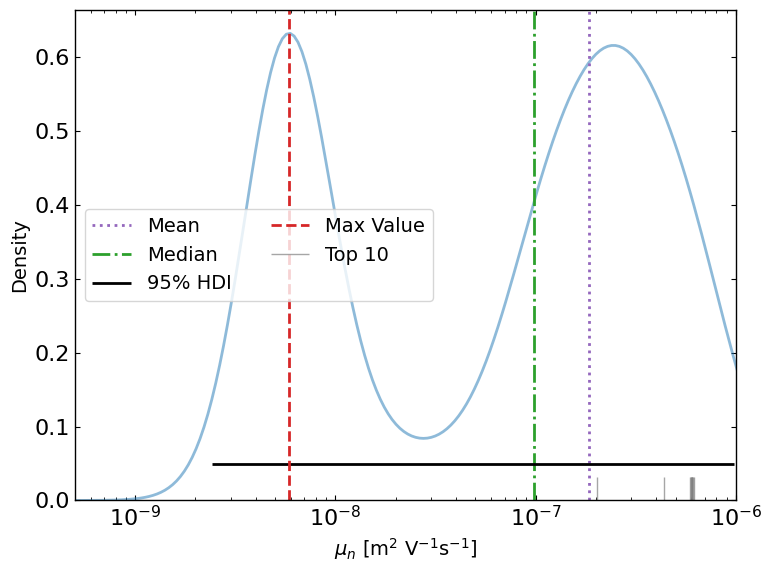
[13]:
from optimpv.posterior.lazy_posterior import LazyPosterior
outcome_name = 'JV_JV_LLH_linear' #optimizer.all_tracking_metrics[0] #'LLH'
data_main = data_main[data_main['trial_index']>=25] # discard the random sampling part
lazy_post = LazyPosterior(params, data_main, outcome_name)
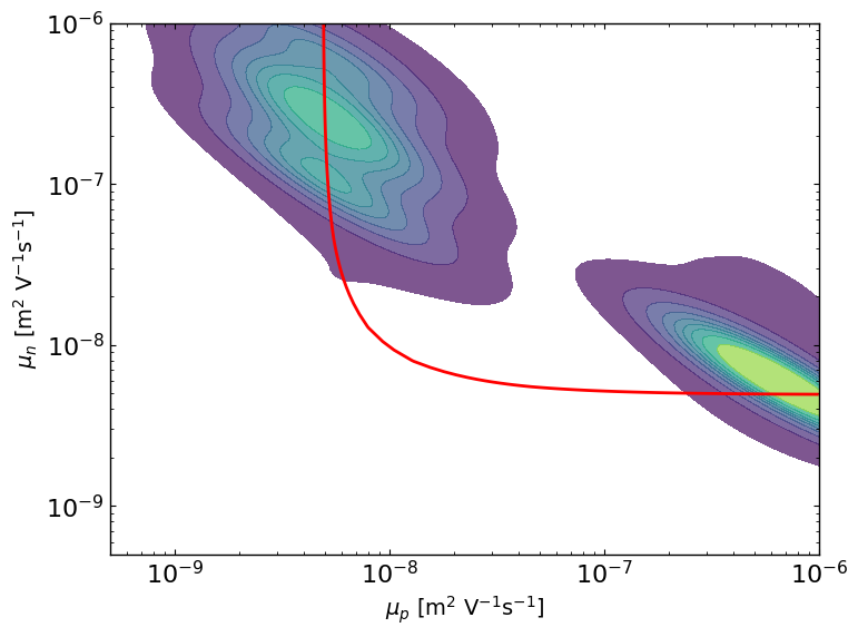
ax8 = lazy_post.plot_lazyposterior_1D_kde('l2.mu_n',title=None,show_top_n=10)
ax9 = lazy_post.plot_lazyposterior_2D_kde('l2.mu_p','l2.mu_n',title=None)
ax9.contour(X_, Y_, Z, levels=[C], colors='r')
plt.show()
[14]:
fig, axes = lazy_post.plot_all_lazyposterior()
[15]:
# Clean up the output files (comment out if you want to keep the output files)
sim.clean_all_output(session_path)
sim.delete_folders('tmp',session_path)
# uncomment the following lines to delete specific files
sim.clean_up_output('ZnO',session_path)
sim.clean_up_output('ActiveLayer',session_path)
sim.clean_up_output('BM_HTL',session_path)
sim.clean_up_output('simulation_setup_fakeOPV',session_path)