Transient absorption spectroscopy fits with rate equation (fake data)
This notebook is a demonstration of how to fit transient absorption spectroscopy (TAS) with the following rate equations:
\[\frac{dn}{dt} = G - k_{trap} n - k_{direct} n^2\]
where \(n\) is the charge carrier density, \(G\) is the generation rate in m⁻³ s⁻¹, ktrap is the trapping rate in s⁻¹, and kdirect is the bimolecular/band-to-bad recombination rate in m³ s⁻¹.
The rate equation described here is the same as employed in the paper by Haffner‐Schirmer et al. 2017 to fit organic solar cell TAS data.
[ ]:
# Import necessary libraries
import warnings, os, sys, copy
# remove warnings from the output
os.environ["PYTHONWARNINGS"] = "ignore"
warnings.filterwarnings(action='ignore', category=FutureWarning)
warnings.filterwarnings(action='ignore', category=UserWarning)
import pandas as pd
import matplotlib.pyplot as plt
import numpy as np
import ax, logging
from ax.utils.notebook.plotting import init_notebook_plotting, render
init_notebook_plotting() # for Jupyter notebooks

try:
    from optimpv import *
    from optimpv.models.RateEqfits.RateEqAgent import RateEqAgent
    from optimpv.models.RateEqfits.RateEqModel import *
    from optimpv.models.RateEqfits.Pumps import *
except Exception as e:
    sys.path.append('../') # add the path to the optimpv module
    from optimpv import *
    from optimpv.models.RateEqfits.RateEqAgent import RateEqAgent
    from optimpv.models.RateEqfits.RateEqModel import *
    from optimpv.models.RateEqfits.Pumps import *
[INFO 12-05 11:49:03] ax.utils.notebook.plotting: Injecting Plotly library into cell. Do not overwrite or delete cell.
[INFO 12-05 11:49:03] ax.utils.notebook.plotting: Please see
    (https://ax.dev/tutorials/visualizations.html#Fix-for-plots-that-are-not-rendering)
    if visualizations are not rendering.
Define the parameters for the simulation
[2]:
# Define the parameters to be fitted
# Note: in general for log spaced value it is better to use the foce_log option when doing the Bayesian optimization
params = []

k_direct = FitParam(name = 'k_direct', value = 1e-16, bounds = [1e-18,1e-14], log_scale = True, rescale = True, value_type = 'float', type='range', display_name=r'$k_{\text{direct}}$', unit='m$^{3}$ s$^{-1}$', axis_type = 'log',force_log=True)
params.append(k_direct)

k_trap = FitParam(name = 'k_trap', value = 1e6, bounds = [1e5,1e7], log_scale = True, rescale = True, value_type = 'float', type='range', display_name=r'$k_{\text{trap}}$', unit='s$^{-1}$', axis_type = 'log',force_log=True)
params.append(k_trap)

cross_section = FitParam(name = 'cross_section', value = 6e-21, bounds = [1e-21,1e-20], log_scale = True, rescale = True, value_type = 'float', type='range', display_name=r'$\sigma$', unit='m$^{2}$', axis_type = 'log',force_log=True)
params.append(cross_section)


# original values
params_orig = copy.deepcopy(params)
num_free_params = 0
dum_dic = {}
for i in range(len(params)):
    if params[i].force_log:
        dum_dic[params[i].name] = np.log10(params[i].value)
    else:
        dum_dic[params[i].name] = params[i].value/params[i].fscale
   # we need this just to run the model to generate some fake data
    if params[i].type != 'fixed'    :
        num_free_params += 1
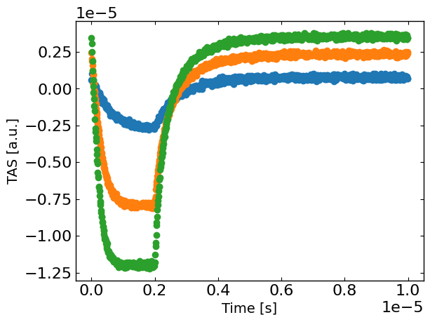
Generate some fake data
Here we generate some fake data to fit. The data is generated using the same model as the one used for the fitting, so it is a good test of the fitting procedure.
[3]:
# Define the necessary input parameters for the model
metric = 'nrmse'
loss = 'linear'
threshold = 10
exp_format = 'TAS'
P = 0.0039 # W
wavelegnth = 850e-9 # m
fpu = 1e5 # Hz
Area = 0.3*0.3*1e-4 # effective pump area in m^-2
penetration_depth = 1e-5*1e-2 # penetration depth in m
pulse_width = 0.2*(1/fpu) # width of the pump pulse in seconds
t0 = 0 # time offset of the pump pulse in seconds
background = 0 # background pump density in m^-3
# Calculate the average absorbed density in photons m^-3
flux, density = get_flux_density(P, wavelegnth, fpu, Area, penetration_depth)
pump_args = {'fpu': fpu , 'pulse_width': pulse_width, 't0': t0, 'P': density, 'background': background, }
fixed_model_args = {'L':100e-9}

t = np.linspace(0,1/fpu,1000)
t = t[:-1]

Gfracs = [0.1,0.5,1]
# concatenate the time and Gfracs
X = None
for Gfrac in Gfracs:
    if X is None:
        X = np.array([t,Gfrac*np.ones(len(t))]).T
    else:
        X = np.concatenate((X,np.array([t,Gfrac*np.ones(len(t))]).T),axis=0)

y_ = X # dummy data

RateEq_fake = RateEqAgent(params, [X], [y_], model = BT_model, pump_model = square_pump, pump_args = pump_args, fixed_model_args = fixed_model_args, metric = metric, loss = loss, threshold=threshold,minimize=True,exp_format=exp_format)

y = RateEq_fake.run(dum_dic,exp_format=exp_format)
noise = 1e-7
from numpy.random import default_rng
rng = default_rng()
y += rng.standard_normal(len(X))*noise

plt.figure()
for idx, Gfrac in enumerate(Gfracs):
    plt.plot(X[X[:,1]==Gfrac,0], y[X[:,1]==Gfrac],'o',label=str(Gfrac),)

plt.xlabel('Time [s]')
plt.ylabel(exp_format + ' [a.u.]')
plt.show()
Run the optimization
[4]:
# Define the Agent and the target metric/loss function
metric = 'nrmse' # can be 'nrmse', 'mse', 'mae'
loss = 'linear' # can be 'linear', 'huber', 'soft_l1'

RateEq = RateEqAgent(params, [X], [y], model = BT_model, pump_model = square_pump, pump_args = pump_args, fixed_model_args = fixed_model_args, metric = metric, loss = loss, threshold=threshold,minimize=True,exp_format=exp_format)
Run the optimization
[ ]:
from optimpv.optimizers.axBOtorch.axBOtorchOptimizer import axBOtorchOptimizer
from optimpv.optimizers.axBOtorch.axUtils import get_VMLC_default_model_kwargs_list

optimizer = axBOtorchOptimizer(params = params, agents = RateEq, models = ['SOBOL','BOTORCH_MODULAR'],n_batches = [1,45], batch_size = [10,2], ax_client = None,  max_parallelism = 100, model_kwargs_list = get_VMLC_default_model_kwargs_list(num_free_params),)
[6]:
# optimizer.optimize() # run the optimization with ax
optimizer.optimize_turbo() # run the optimization with turbo
[INFO 12-05 11:49:04] optimpv.axBOtorchOptimizer: Starting optimization with 46 batches and a total of 100 trials
[INFO 12-05 11:49:04] optimpv.axBOtorchOptimizer: Starting Sobol batch 1 with 10 trials
[INFO 12-05 11:49:05] optimpv.axBOtorchOptimizer: Finished Sobol with best value of 0.049954
[INFO 12-05 11:49:06] optimpv.axBOtorchOptimizer: Finished Turbo batch 2 with 2 trials with current best value: 5.00e-02, TR length: 5.00e-01
[INFO 12-05 11:49:06] optimpv.axBOtorchOptimizer: Finished Turbo batch 3 with 2 trials with current best value: 5.00e-02, TR length: 5.00e-01
[INFO 12-05 11:49:07] optimpv.axBOtorchOptimizer: Finished Turbo batch 4 with 2 trials with current best value: 5.00e-02, TR length: 3.12e-01
[INFO 12-05 11:49:07] optimpv.axBOtorchOptimizer: Finished Turbo batch 5 with 2 trials with current best value: 5.00e-02, TR length: 3.12e-01
[INFO 12-05 11:49:07] optimpv.axBOtorchOptimizer: Finished Turbo batch 6 with 2 trials with current best value: 5.00e-02, TR length: 1.95e-01
[INFO 12-05 11:49:07] optimpv.axBOtorchOptimizer: Finished Turbo batch 7 with 2 trials with current best value: 4.73e-02, TR length: 1.95e-01
[INFO 12-05 11:49:07] optimpv.axBOtorchOptimizer: Finished Turbo batch 8 with 2 trials with current best value: 4.73e-02, TR length: 1.95e-01
[INFO 12-05 11:49:08] optimpv.axBOtorchOptimizer: Finished Turbo batch 9 with 2 trials with current best value: 3.98e-02, TR length: 1.95e-01
[INFO 12-05 11:49:08] optimpv.axBOtorchOptimizer: Finished Turbo batch 10 with 2 trials with current best value: 3.98e-02, TR length: 1.95e-01
[INFO 12-05 11:49:08] optimpv.axBOtorchOptimizer: Finished Turbo batch 11 with 2 trials with current best value: 3.47e-02, TR length: 1.95e-01
[INFO 12-05 11:49:08] optimpv.axBOtorchOptimizer: Finished Turbo batch 12 with 2 trials with current best value: 3.47e-02, TR length: 1.95e-01
[INFO 12-05 11:49:08] optimpv.axBOtorchOptimizer: Finished Turbo batch 13 with 2 trials with current best value: 3.47e-02, TR length: 1.22e-01
[INFO 12-05 11:49:09] optimpv.axBOtorchOptimizer: Finished Turbo batch 14 with 2 trials with current best value: 3.17e-02, TR length: 1.22e-01
[INFO 12-05 11:49:09] optimpv.axBOtorchOptimizer: Finished Turbo batch 15 with 2 trials with current best value: 2.61e-02, TR length: 1.22e-01
[INFO 12-05 11:49:09] optimpv.axBOtorchOptimizer: Finished Turbo batch 16 with 2 trials with current best value: 2.61e-02, TR length: 1.22e-01
[INFO 12-05 11:49:09] optimpv.axBOtorchOptimizer: Finished Turbo batch 17 with 2 trials with current best value: 2.16e-02, TR length: 1.22e-01
[INFO 12-05 11:49:09] optimpv.axBOtorchOptimizer: Finished Turbo batch 18 with 2 trials with current best value: 2.16e-02, TR length: 1.22e-01
[INFO 12-05 11:49:10] optimpv.axBOtorchOptimizer: Finished Turbo batch 19 with 2 trials with current best value: 2.12e-02, TR length: 1.22e-01
[INFO 12-05 11:49:10] optimpv.axBOtorchOptimizer: Finished Turbo batch 20 with 2 trials with current best value: 1.95e-02, TR length: 1.22e-01
[INFO 12-05 11:49:10] optimpv.axBOtorchOptimizer: Finished Turbo batch 21 with 2 trials with current best value: 1.83e-02, TR length: 1.95e-01
[INFO 12-05 11:49:10] optimpv.axBOtorchOptimizer: Finished Turbo batch 22 with 2 trials with current best value: 1.83e-02, TR length: 1.95e-01
[INFO 12-05 11:49:10] optimpv.axBOtorchOptimizer: Finished Turbo batch 23 with 2 trials with current best value: 1.83e-02, TR length: 1.22e-01
[INFO 12-05 11:49:10] optimpv.axBOtorchOptimizer: Finished Turbo batch 24 with 2 trials with current best value: 9.19e-03, TR length: 1.22e-01
[INFO 12-05 11:49:11] optimpv.axBOtorchOptimizer: Finished Turbo batch 25 with 2 trials with current best value: 9.19e-03, TR length: 1.22e-01
[INFO 12-05 11:49:11] optimpv.axBOtorchOptimizer: Finished Turbo batch 26 with 2 trials with current best value: 9.19e-03, TR length: 7.63e-02
[INFO 12-05 11:49:11] optimpv.axBOtorchOptimizer: Finished Turbo batch 27 with 2 trials with current best value: 9.19e-03, TR length: 7.63e-02
[INFO 12-05 11:49:11] optimpv.axBOtorchOptimizer: Finished Turbo batch 28 with 2 trials with current best value: 9.19e-03, TR length: 4.77e-02
[INFO 12-05 11:49:11] optimpv.axBOtorchOptimizer: Finished Turbo batch 29 with 2 trials with current best value: 8.81e-03, TR length: 4.77e-02
[INFO 12-05 11:49:12] optimpv.axBOtorchOptimizer: Finished Turbo batch 30 with 2 trials with current best value: 7.57e-03, TR length: 4.77e-02
[INFO 12-05 11:49:12] optimpv.axBOtorchOptimizer: Finished Turbo batch 31 with 2 trials with current best value: 7.57e-03, TR length: 4.77e-02
[INFO 12-05 11:49:12] optimpv.axBOtorchOptimizer: Finished Turbo batch 32 with 2 trials with current best value: 7.57e-03, TR length: 2.98e-02
[INFO 12-05 11:49:12] optimpv.axBOtorchOptimizer: Finished Turbo batch 33 with 2 trials with current best value: 7.57e-03, TR length: 2.98e-02
[INFO 12-05 11:49:12] optimpv.axBOtorchOptimizer: Finished Turbo batch 34 with 2 trials with current best value: 7.57e-03, TR length: 1.86e-02
[INFO 12-05 11:49:13] optimpv.axBOtorchOptimizer: Finished Turbo batch 35 with 2 trials with current best value: 7.57e-03, TR length: 1.86e-02
[INFO 12-05 11:49:13] optimpv.axBOtorchOptimizer: Finished Turbo batch 36 with 2 trials with current best value: 7.57e-03, TR length: 1.16e-02
[INFO 12-05 11:49:13] optimpv.axBOtorchOptimizer: Finished Turbo batch 37 with 2 trials with current best value: 7.37e-03, TR length: 1.16e-02
[INFO 12-05 11:49:13] optimpv.axBOtorchOptimizer: Finished Turbo batch 38 with 2 trials with current best value: 6.98e-03, TR length: 1.16e-02
[INFO 12-05 11:49:13] optimpv.axBOtorchOptimizer: Finished Turbo batch 39 with 2 trials with current best value: 6.98e-03, TR length: 1.16e-02
[INFO 12-05 11:49:13] optimpv.axBOtorchOptimizer: Finished Turbo batch 40 with 2 trials with current best value: 6.98e-03, TR length: 7.28e-03
[INFO 12-05 11:49:14] optimpv.axBOtorchOptimizer: Turbo converged after 40 batches with 80 trials
[7]:
# get the best parameters and update the params list in the optimizer and the agent
ax_client = optimizer.ax_client # get the ax client
optimizer.update_params_with_best_balance() # update the params list in the optimizer with the best parameters
RateEq.params = optimizer.params # update the params list in the agent with the best parameters

# print the best parameters
print('Best parameters:')
for p,po in zip(optimizer.params, params_orig):
    print(p.name, 'fitted value:', p.value, 'original value:', po.value)
Best parameters:
k_direct fitted value: 9.578473450624297e-17 original value: 1e-16
k_trap fitted value: 1120423.3472038193 original value: 1000000.0
cross_section fitted value: 6.0145951309540925e-21 original value: 6e-21
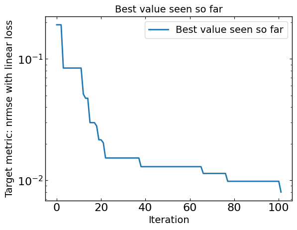
[8]:
# Plot optimization results
data = ax_client.summarize()
all_metrics = optimizer.all_metrics
plt.figure()
plt.plot(np.minimum.accumulate(data[all_metrics]), label="Best value seen so far")
plt.yscale("log")
plt.xlabel("Iteration")
plt.ylabel("Target metric: " + metric + " with " + loss + " loss")
plt.legend()
plt.title("Best value seen so far")

print("Best value seen so far is ", min(data[all_metrics[0]]), "at iteration ", int(data[all_metrics[0]].idxmin()))
plt.show()
Best value seen so far is 0.006981551313823108 at iteration 83
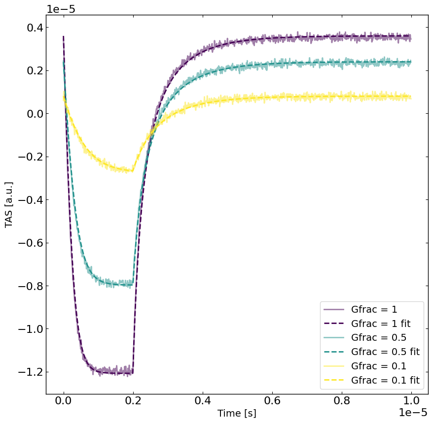
[9]:
# rerun the simulation with the best parameters
yfit = RateEq.run(parameters={},exp_format=exp_format) # run the simulation with the best parameters

viridis = plt.get_cmap('viridis', len(Gfracs))
plt.figure(figsize=(10,10))
linewidth = 2
for idx, Gfrac in enumerate(Gfracs[::-1]):
    plt.plot(X[X[:,1]==Gfrac,0],y[X[:,1]==Gfrac],label='Gfrac = '+str(Gfrac),color=viridis(idx),alpha=0.5,linewidth=linewidth)
    plt.plot(X[X[:,1]==Gfrac,0],yfit[X[:,1]==Gfrac],label='Gfrac = '+str(Gfrac)+' fit',linestyle='--',color=viridis(idx),linewidth=linewidth)
plt.xlabel('Time [s]')
plt.ylabel(exp_format + ' [a.u.]')
plt.legend()
plt.show()