Design of Experiment: Optimize perovskite solar cells efficiency

This notebook is made to use optimPV for experimental design. Here, we show how to load some data from a presampling, and how to use optimPV to suggest the next set of experiment using Bayesian optimization. The goal here is to optimize the processing conditions for a perovskite solar cell to maximize the power conversion efficiency (PCE).

Note: The data used here is real data generated in the i-MEET and HI-ERN labs at the university of Erlangen-Nuremberg (FAU) by Jiyun Zhang for the paper: Autonomous Optimization of Air-Processed Perovskite Solar Cell in a 6D Parameter Space

# Import necessary libraries
import warnings, os, sys, shutil
# remove warnings from the output
os.environ["PYTHONWARNINGS"] = "ignore"
warnings.filterwarnings(action='ignore', category=FutureWarning)
warnings.filterwarnings(action='ignore', category=UserWarning)
import pandas as pd
import matplotlib.pyplot as plt
import numpy as np
from numpy.random import default_rng
import torch, copy, uuid
import pySIMsalabim as sim
from pySIMsalabim.experiments.JV_steady_state import *
import ax, logging
from ax.utils.notebook.plotting import init_notebook_plotting, render
init_notebook_plotting() # for Jupyter notebooks

try:
    from optimpv import *
    from optimpv.axBOtorch.axUtils import *
except Exception as e:
    sys.path.append('../') # add the path to the optimpv module
    from optimpv import *
    from optimpv.axBOtorch.axUtils import *

[INFO 08-13 17:25:42] ax.utils.notebook.plotting: Injecting Plotly library into cell. Do not overwrite or delete cell.
[INFO 08-13 17:25:42] ax.utils.notebook.plotting: Please see
    (https://ax.dev/tutorials/visualizations.html#Fix-for-plots-that-are-not-rendering)
    if visualizations are not rendering.

Get the data

# Define the path to the data
data_dir =os.path.join(os.path.abspath('../'),'Data','6D_pero_opti') # path to the data directory

# Load the data
df = pd.read_csv(os.path.join(data_dir,'6D_pero_opti.csv'),sep=r'\s+') # load the data

# Display some information about the data
print(df.describe())

       Spin_Speed_1  Duration_t1  Spin_Speed_2  Dispense_Speed  Duration_t3  \
count     76.000000    76.000000     76.000000       76.000000    76.000000
mean    1520.486842    18.276316   2273.289474      234.697368    17.315789
std      458.510240     7.000188    501.488845       83.133470     7.919950
min      540.000000     5.000000   1021.000000       16.000000     5.000000
25%     1203.500000    13.750000   2019.500000      201.750000    10.750000
50%     1511.000000    18.000000   2385.500000      247.500000    17.000000
75%     1801.250000    22.000000   2671.000000      277.500000    23.250000
max     2579.000000    34.000000   3000.000000      396.000000    35.000000

       Spin_Speed_3        Jsc        Voc         FF       Pmax       Vmpp  \
count     76.000000  76.000000  76.000000  76.000000  76.000000  76.000000
mean    3717.789474  24.391395   1.021157   0.724692  18.320711   0.825778
std      917.207346   1.872929   0.108197   0.055290   3.486546   0.105413
min     2000.000000  12.231000   0.616300   0.448800   4.690000   0.463000
25%     3002.000000  24.173500   0.987650   0.704400  17.477000   0.785750
50%     3825.000000  24.615000   1.038750   0.734700  18.851500   0.835000
75%     4471.500000  25.279500   1.100725   0.759925  20.347250   0.895000
max     5000.000000  25.938000   1.162200   0.810900  23.729000   0.990100

           Rseries       Rshunt
count    76.000000    76.000000
mean   3720.112882  2763.793289
std    1487.516713  1956.263177
min      92.129000     2.990000
25%    3146.452500   228.750000
50%    3739.157000  3290.000000
75%    4567.406250  4285.000000
max    6513.151000  6860.000000

Define the parameters for the simulation

params = [] # list of parameters to be optimized

Spin_Speed_1 = FitParam(name = 'Spin_Speed_1', value = 1000, bounds = [500,3000], value_type = 'int', display_name='Spin Speed 1', unit='rpm', axis_type = 'linear')
params.append(Spin_Speed_1)

Duration_t1 = FitParam(name = 'Duration_t1', value = 10, bounds = [5,35], value_type = 'int', display_name='Duration t1', unit='s', axis_type = 'linear')
params.append(Duration_t1)

Spin_Speed_2 = FitParam(name = 'Spin_Speed_2', value = 1000, bounds = [1000,3000], value_type = 'int', display_name='Spin Speed 2', unit='rpm', axis_type = 'linear')
params.append(Spin_Speed_2)

Dispense_Speed = FitParam(name = 'Dispense_Speed', value = 100, bounds = [10,400], value_type = 'int', display_name='Dispense Speed', unit='rpm', axis_type = 'linear')
params.append(Dispense_Speed)

Duration_t3 = FitParam(name = 'Duration_t3', value = 10, bounds = [5,35], value_type = 'int', display_name='Duration t3', unit='s', axis_type = 'linear')
params.append(Duration_t3)

Spin_Speed_3 = FitParam(name = 'Spin_Speed_3', value = 3000, bounds = [2000,5000], value_type = 'int', display_name='Spin Speed 3', unit='rpm', axis_type = 'linear')
params.append(Spin_Speed_3)

Run the optimization

# Define the Agent and the target metric/loss function
from optimpv.general.SuggestOnlyAgent import SuggestOnlyAgent

suggest = SuggestOnlyAgent(params,exp_format='Pmax',minimize=False,tracking_exp_format=['Jsc','Voc','FF'],name=None)

from optimpv.axBOtorch.axBOtorchOptimizer import axBOtorchOptimizer
from botorch.acquisition.logei import qLogNoisyExpectedImprovement
from ax.adapter.transforms.standardize_y import StandardizeY
from ax.adapter.transforms.unit_x import UnitX
from ax.adapter.transforms.remove_fixed import RemoveFixed
from ax.adapter.transforms.log import Log
from ax.generators.torch.botorch_modular.utils import ModelConfig
from ax.generators.torch.botorch_modular.surrogate import SurrogateSpec
from gpytorch.kernels import MaternKernel
from gpytorch.kernels import ScaleKernel
from botorch.models import SingleTaskGP
from botorch.models.map_saas import AdditiveMapSaasSingleTaskGP
from botorch.models.fully_bayesian import SaasFullyBayesianSingleTaskGP
model_gen_kwargs_list = None
parameter_constraints = None

model_kwargs_list = [{"torch_device":torch.device("cuda" if torch.cuda.is_available() else "cpu"),'botorch_acqf_class':qLogNoisyExpectedImprovement,'transforms':[RemoveFixed, Log, UnitX, StandardizeY],'surrogate_spec':SurrogateSpec(model_configs=[ModelConfig(botorch_model_class=SaasFullyBayesianSingleTaskGP,covar_module_class=ScaleKernel, covar_module_options={'base_kernel':MaternKernel(nu=2.5, ard_num_dims=len(params))})])}]
model_kwargs_list =None

# Define the optimizer
optimizer = axBOtorchOptimizer(params = params, agents = suggest, models = ['BOTORCH_MODULAR'],n_batches = [1], batch_size = [6], ax_client = None,  max_parallelism = -1, model_kwargs_list = model_kwargs_list, model_gen_kwargs_list = None, name = 'ax_opti',suggest_only = True,existing_data=df,verbose_logging=True)

# Run the optimization
best_value_previous_step = 22.973
kwargs_turbo_state = {'length': 0.4, 'success_counter': 1, 'failure_counter': 1 }
turbo_state_params = optimizer.optimize_turbo(kwargs_turbo={"best_value": best_value_previous_step}, kwargs_turbo_state=kwargs_turbo_state) # run the optimization with turbo
# The current state of the turbo optimization is stored in the kwargs_turbo_state parameter, which can be used to continue the optimization in the next step

[INFO 08-13 17:25:43] optimpv.axBOtorchOptimizer: Starting optimization with 1 batches and a total of 6 trials
[INFO 08-13 17:25:43] optimpv.axBOtorchOptimizer: Using existing data for initialization
[INFO 08-13 17:25:43] optimpv.axBOtorchOptimizer: Suggesting 6 trials without running the agents.
[WARNING 08-13 17:25:44] ax.api.client: Metric IMetric('Jsc') not found in optimization config, added as tracking metric.
[WARNING 08-13 17:25:44] ax.api.client: Metric IMetric('Voc') not found in optimization config, added as tracking metric.
[WARNING 08-13 17:25:44] ax.api.client: Metric IMetric('FF') not found in optimization config, added as tracking metric.
[INFO 08-13 17:25:44] ax.api.client: Trial 0 marked COMPLETED.
[INFO 08-13 17:25:44] ax.api.client: Trial 1 marked COMPLETED.
[INFO 08-13 17:25:44] ax.api.client: Trial 2 marked COMPLETED.
[INFO 08-13 17:25:44] ax.api.client: Trial 3 marked COMPLETED.
[INFO 08-13 17:25:44] ax.api.client: Trial 4 marked COMPLETED.
[INFO 08-13 17:25:44] ax.api.client: Trial 5 marked COMPLETED.
[INFO 08-13 17:25:44] ax.api.client: Trial 6 marked COMPLETED.
[INFO 08-13 17:25:44] ax.api.client: Trial 7 marked COMPLETED.
[INFO 08-13 17:25:44] ax.api.client: Trial 8 marked COMPLETED.
[INFO 08-13 17:25:44] ax.api.client: Trial 9 marked COMPLETED.
[INFO 08-13 17:25:44] ax.api.client: Trial 10 marked COMPLETED.
[INFO 08-13 17:25:44] ax.api.client: Trial 11 marked COMPLETED.
[INFO 08-13 17:25:44] ax.api.client: Trial 12 marked COMPLETED.
[INFO 08-13 17:25:44] ax.api.client: Trial 13 marked COMPLETED.
[INFO 08-13 17:25:44] ax.api.client: Trial 14 marked COMPLETED.
[INFO 08-13 17:25:44] ax.api.client: Trial 15 marked COMPLETED.
[INFO 08-13 17:25:44] ax.api.client: Trial 16 marked COMPLETED.
[INFO 08-13 17:25:44] ax.api.client: Trial 17 marked COMPLETED.
[INFO 08-13 17:25:44] ax.api.client: Trial 18 marked COMPLETED.
[INFO 08-13 17:25:44] ax.api.client: Trial 19 marked COMPLETED.
[INFO 08-13 17:25:44] ax.api.client: Trial 20 marked COMPLETED.
[INFO 08-13 17:25:44] ax.api.client: Trial 21 marked COMPLETED.
[INFO 08-13 17:25:44] ax.api.client: Trial 22 marked COMPLETED.
[INFO 08-13 17:25:44] ax.api.client: Trial 23 marked COMPLETED.
[INFO 08-13 17:25:44] ax.api.client: Trial 24 marked COMPLETED.
[INFO 08-13 17:25:44] ax.api.client: Trial 25 marked COMPLETED.
[INFO 08-13 17:25:44] ax.api.client: Trial 26 marked COMPLETED.
[INFO 08-13 17:25:44] ax.api.client: Trial 27 marked COMPLETED.
[INFO 08-13 17:25:44] ax.api.client: Trial 28 marked COMPLETED.
[INFO 08-13 17:25:44] ax.api.client: Trial 29 marked COMPLETED.
[INFO 08-13 17:25:44] ax.api.client: Trial 30 marked COMPLETED.
[INFO 08-13 17:25:44] ax.api.client: Trial 31 marked COMPLETED.
[INFO 08-13 17:25:44] ax.api.client: Trial 32 marked COMPLETED.
[INFO 08-13 17:25:44] ax.api.client: Trial 33 marked COMPLETED.
[INFO 08-13 17:25:44] ax.api.client: Trial 34 marked COMPLETED.
[INFO 08-13 17:25:44] ax.api.client: Trial 35 marked COMPLETED.
[INFO 08-13 17:25:44] ax.api.client: Trial 36 marked COMPLETED.
[INFO 08-13 17:25:44] ax.api.client: Trial 37 marked COMPLETED.
[INFO 08-13 17:25:44] ax.api.client: Trial 38 marked COMPLETED.
[INFO 08-13 17:25:44] ax.api.client: Trial 39 marked COMPLETED.
[INFO 08-13 17:25:44] ax.api.client: Trial 40 marked COMPLETED.
[INFO 08-13 17:25:44] ax.api.client: Trial 41 marked COMPLETED.
[INFO 08-13 17:25:44] ax.api.client: Trial 42 marked COMPLETED.
[INFO 08-13 17:25:44] ax.api.client: Trial 43 marked COMPLETED.
[INFO 08-13 17:25:44] ax.api.client: Trial 44 marked COMPLETED.
[INFO 08-13 17:25:44] ax.api.client: Trial 45 marked COMPLETED.
[INFO 08-13 17:25:44] ax.api.client: Trial 46 marked COMPLETED.
[INFO 08-13 17:25:44] ax.api.client: Trial 47 marked COMPLETED.
[INFO 08-13 17:25:44] ax.api.client: Trial 48 marked COMPLETED.
[INFO 08-13 17:25:44] ax.api.client: Trial 49 marked COMPLETED.
[INFO 08-13 17:25:44] ax.api.client: Trial 50 marked COMPLETED.
[INFO 08-13 17:25:44] ax.api.client: Trial 51 marked COMPLETED.
[INFO 08-13 17:25:44] ax.api.client: Trial 52 marked COMPLETED.
[INFO 08-13 17:25:44] ax.api.client: Trial 53 marked COMPLETED.
[INFO 08-13 17:25:44] ax.api.client: Trial 54 marked COMPLETED.
[INFO 08-13 17:25:44] ax.api.client: Trial 55 marked COMPLETED.
[INFO 08-13 17:25:44] ax.api.client: Trial 56 marked COMPLETED.
[INFO 08-13 17:25:44] ax.api.client: Trial 57 marked COMPLETED.
[INFO 08-13 17:25:44] ax.api.client: Trial 58 marked COMPLETED.
[INFO 08-13 17:25:44] ax.api.client: Trial 59 marked COMPLETED.
[INFO 08-13 17:25:44] ax.api.client: Trial 60 marked COMPLETED.
[INFO 08-13 17:25:44] ax.api.client: Trial 61 marked COMPLETED.
[INFO 08-13 17:25:44] ax.api.client: Trial 62 marked COMPLETED.
[INFO 08-13 17:25:44] ax.api.client: Trial 63 marked COMPLETED.
[INFO 08-13 17:25:44] ax.api.client: Trial 64 marked COMPLETED.
[INFO 08-13 17:25:44] ax.api.client: Trial 65 marked COMPLETED.
[INFO 08-13 17:25:44] ax.api.client: Trial 66 marked COMPLETED.
[INFO 08-13 17:25:44] ax.api.client: Trial 67 marked COMPLETED.
[INFO 08-13 17:25:44] ax.api.client: Trial 68 marked COMPLETED.
[INFO 08-13 17:25:44] ax.api.client: Trial 69 marked COMPLETED.
[INFO 08-13 17:25:44] ax.api.client: Trial 70 marked COMPLETED.
[INFO 08-13 17:25:44] ax.api.client: Trial 71 marked COMPLETED.
[INFO 08-13 17:25:44] ax.api.client: Trial 72 marked COMPLETED.
[INFO 08-13 17:25:44] ax.api.client: Trial 73 marked COMPLETED.
[INFO 08-13 17:25:44] ax.api.client: Trial 74 marked COMPLETED.
[INFO 08-13 17:25:44] ax.api.client: Trial 75 marked COMPLETED.
[INFO 08-13 17:25:44] optimpv.axBOtorchOptimizer: Suggesting 6 trials without running the agents

# get the best parameters and update the params list in the optimizer and the agent
ax_client = optimizer.ax_client # get the ax client
optimizer.update_params_with_best_balance() # update the params list in the optimizer with the best parameters
suggest.params = optimizer.params # update the params list in the agent with the best parameters

print("Best parameters found:")
for p in optimizer.params:
    print(f"{p.name}: {p.value} {p.unit} ")

Best parameters found:
Spin_Speed_1: 1165 rpm
Duration_t1: 23 s
Spin_Speed_2: 2063 rpm
Dispense_Speed: 241 rpm
Duration_t3: 32 s
Spin_Speed_3: 2863 rpm

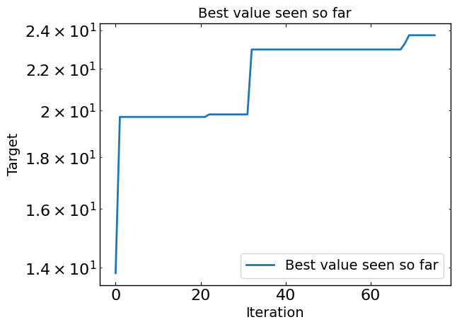
# Plot optimization results
data = ax_client.summarize()
all_metrics = optimizer.all_metrics
plt.figure()
plt.plot(np.maximum.accumulate(data[all_metrics]), label="Best value seen so far")
plt.yscale("log")
plt.xlabel("Iteration")
plt.ylabel("Target")
plt.legend()
plt.title("Best value seen so far")

print("Best value seen so far is ", max(data[all_metrics[0]]), "at iteration ", int(data[all_metrics[0]].idxmin()))

plt.show()

Best value seen so far is  23.729 at iteration  27

# print the parameters to that are running in data
to_run_next = data[data['trial_status'] == 'RUNNING']
print("Parameters to run next:")
print(to_run_next)

Parameters to run next:
    trial_index arm_name trial_status  Jsc  Voc  FF  Pmax  Spin_Speed_1  \
76           76     76_0      RUNNING  NaN  NaN NaN   NaN           995
77           77     77_0      RUNNING  NaN  NaN NaN   NaN          1026
78           78     78_0      RUNNING  NaN  NaN NaN   NaN          1229
79           79     79_0      RUNNING  NaN  NaN NaN   NaN          1008
80           80     80_0      RUNNING  NaN  NaN NaN   NaN          1044
81           81     81_0      RUNNING  NaN  NaN NaN   NaN           988

    Duration_t1  Spin_Speed_2  Dispense_Speed  Duration_t3  Spin_Speed_3
76           29          1893             199           25          2680
77           31          2039             281           29          2535
78           32          2026             263           22          2597
79           33          1949             197           30          2582
80           31          1973             192           21          2760
81           33          2049             189           26          2676

cards = ax_client.compute_analyses(display=True)

Overview of the Entire Optimization Process

This analysis provides an overview of the entire optimization process. It includes visualizations of the results obtained so far, insights into the parameter and metric relationships learned by the Ax model, diagnostics such as model fit, and health checks to assess the overall health of the experiment.

Results Analysis

Result Analyses provide a high-level overview of the results of the optimization process so far with respect to the metrics specified in experiment design.

Metric Effects: Predicted and observed effects for all arms in the experiment

These pair of plots visualize the metric effects for each arm, with the Ax model predictions on the left and the raw observed data on the right. The predicted effects apply shrinkage for noise and adjust for non-stationarity in the data, so they are more representative of the reproducible effects that will manifest in a long-term validation experiment.

Metric Effects Pair for Pmax

Modeled Arm Effects on Pmax

Modeled effects on Pmax. This plot visualizes predictions of the true metric changes for each arm based on Ax's model. This is the expected delta you would expect if you (re-)ran that arm. This plot helps in anticipating the outcomes and performance of arms based on the model's predictions. Note, flat predictions across arms indicate that the model predicts that there is no effect, meaning if you were to re-run the experiment, the delta you would see would be small and fall within the confidence interval indicated in the plot.

Observed Arm Effects on Pmax

Observed effects on Pmax. This plot visualizes the effects from previously-run arms on a specific metric, providing insights into their performance. This plot allows one to compare and contrast the effectiveness of different arms, highlighting which configurations have yielded the most favorable outcomes.

Summary for ax_opti

High-level summary of the `Trial`-s in this `Experiment`

	trial_index	arm_name	trial_status	Jsc	Voc	FF	Pmax	Spin_Speed_1	Duration_t1	Spin_Speed_2	Dispense_Speed	Duration_t3	Spin_Speed_3
0	0	0_0	COMPLETED	24.507	0.9100	0.6201	13.830	2404	15	1745	203	13	4494
1	1	1_0	COMPLETED	25.733	1.0090	0.7592	19.712	1835	17	2289	289	11	4389
2	2	2_0	COMPLETED	24.692	1.0321	0.7376	18.797	1067	33	2352	234	5	2861
3	3	3_0	COMPLETED	24.195	0.8197	0.6506	12.903	2276	18	1821	26	15	3241
4	4	4_0	COMPLETED	24.268	0.9951	0.7684	18.556	2147	30	2816	290	29	4981
5	5	5_0	COMPLETED	24.481	1.0100	0.7264	17.962	1152	28	2734	121	8	4856
6	6	6_0	COMPLETED	25.575	0.9926	0.7377	18.726	1240	23	2993	190	19	2560
7	7	7_0	COMPLETED	23.995	0.6850	0.6336	10.414	2471	21	1394	138	29	2046
8	8	8_0	COMPLETED	24.283	0.9940	0.7185	17.342	907	9	2766	314	22	4323
9	9	9_0	COMPLETED	12.231	0.8321	0.5819	5.922	2034	18	1021	90	7	4776
10	10	10_0	COMPLETED	23.558	0.9297	0.6919	15.154	540	19	2383	16	23	4632
11	11	11_0	COMPLETED	25.214	0.9921	0.7637	19.105	1532	12	1955	383	18	4137
12	12	12_0	COMPLETED	24.944	1.0080	0.7018	17.644	1024	8	2631	367	21	2135
13	13	13_0	COMPLETED	24.301	1.0172	0.7420	18.340	1768	22	2927	77	10	4208
14	14	14_0	COMPLETED	23.929	0.9692	0.6905	16.013	1598	29	2592	396	23	3688
15	15	15_0	COMPLETED	24.251	0.9949	0.6952	16.773	691	14	1661	248	19	3523
16	16	16_0	COMPLETED	20.114	0.6694	0.5930	7.984	1745	28	1098	108	16	2467
17	17	17_0	COMPLETED	25.454	0.9170	0.7359	17.178	2111	31	2065	349	27	2251
18	18	18_0	COMPLETED	25.549	0.9484	0.7094	17.190	621	26	1221	51	26	3907
19	19	19_0	COMPLETED	24.824	0.9231	0.8109	18.583	1442	9	1297	306	9	3972
20	20	20_0	COMPLETED	24.913	0.8165	0.7027	14.294	810	33	1776	258	6	4599
21	21	21_0	COMPLETED	24.870	0.9743	0.7497	18.165	1308	32	2558	146	12	3111
22	22	22_0	COMPLETED	25.625	1.0253	0.7546	19.824	1333	20	1878	212	24	3386
23	23	23_0	COMPLETED	25.641	1.0022	0.7049	18.115	863	34	1535	104	25	3160
24	24	24_0	COMPLETED	24.788	0.9533	0.7081	16.732	675	26	1604	66	21	2720
25	25	25_0	COMPLETED	24.213	1.0209	0.7637	18.876	1420	12	2015	277	7	3621
26	26	26_0	COMPLETED	24.022	0.9163	0.7127	15.688	1972	24	2137	218	16	2822
27	27	27_0	COMPLETED	16.955	0.6163	0.4488	4.690	2349	15	1315	35	18	2282
28	28	28_0	COMPLETED	24.370	0.9586	0.7501	17.522	2211	10	2465	156	13	2585
29	29	29_0	COMPLETED	24.711	1.0388	0.7582	19.463	1632	20	2233	328	14	3025
30	30	30_0	COMPLETED	23.312	0.9011	0.6478	13.608	1881	25	1449	360	10	3843
31	31	31_0	COMPLETED	23.852	0.9480	0.7195	16.270	953	13	1167	177	27	3463
32	32	32_0	COMPLETED	25.429	1.1523	0.7840	22.973	1474	14	2324	250	19	3910
33	33	33_0	COMPLETED	24.912	1.1458	0.7811	22.298	1515	16	2676	269	6	3552
34	34	34_0	COMPLETED	25.132	1.1228	0.7614	21.484	1165	23	2063	241	32	2863
35	35	35_0	COMPLETED	25.680	1.0820	0.7335	20.381	1913	13	2671	221	22	5000
36	36	36_0	COMPLETED	24.773	1.0860	0.7178	19.312	1421	8	2021	279	25	3002
37	37	37_0	COMPLETED	24.990	1.0630	0.7175	19.060	1840	5	2401	360	10	3825
38	38	38_0	COMPLETED	25.533	1.0700	0.7514	20.529	1476	13	2036	242	25	5000
39	39	39_0	COMPLETED	24.830	1.0592	0.7310	19.226	1096	20	2295	246	17	2231
40	40	40_0	COMPLETED	25.093	1.1027	0.7718	21.355	2126	21	2903	266	9	5000
41	41	41_0	COMPLETED	24.613	1.1195	0.7264	20.017	1600	18	2444	187	32	4233
42	42	42_0	COMPLETED	24.369	1.0772	0.6713	17.623	1184	29	1946	191	35	4204
43	43	43_0	COMPLETED	23.966	1.1008	0.6978	18.409	1210	18	1933	325	21	2000
44	44	44_0	COMPLETED	23.437	1.0966	0.7084	18.206	1220	15	2546	198	11	2783
45	45	45_0	COMPLETED	24.425	1.1057	0.7500	20.256	1570	5	2329	210	19	4466
46	46	46_0	COMPLETED	24.617	1.0551	0.6368	16.540	925	22	2808	268	5	2000
47	47	47_0	COMPLETED	23.938	1.1056	0.7443	19.700	1631	22	2902	281	5	3450
48	48	48_0	COMPLETED	24.050	0.9692	0.6917	16.123	1720	5	2707	260	10	4488
49	49	49_0	COMPLETED	23.916	1.1053	0.7251	19.168	1451	9	2149	256	27	3416
50	50	50_0	COMPLETED	24.857	1.1243	0.7888	22.046	2358	19	2981	298	13	3658
51	51	51_0	COMPLETED	24.510	1.0840	0.7587	20.158	1490	19	2611	270	5	4888
52	52	52_0	COMPLETED	23.600	1.1120	0.7749	20.336	1790	20	2696	227	5	5000
53	53	53_0	COMPLETED	23.336	1.0387	0.7318	17.739	1120	18	2238	273	31	3881
54	54	54_0	COMPLETED	24.658	1.1007	0.7607	20.647	1509	18	2552	254	17	4265
55	55	55_0	COMPLETED	24.566	1.0401	0.7475	19.101	1317	18	2336	262	23	4092
56	56	56_0	COMPLETED	24.468	1.1097	0.7705	20.922	1671	16	2613	271	17	3640
57	57	57_0	COMPLETED	24.306	1.0880	0.7490	19.808	1596	19	2668	237	12	4999
58	58	58_0	COMPLETED	23.984	1.0320	0.7191	17.798	1428	15	2488	292	13	4281
59	59	59_0	COMPLETED	24.109	1.0785	0.7565	19.671	1513	15	2388	198	18	4580
60	60	60_0	COMPLETED	24.934	1.1210	0.7600	21.242	2134	20	2989	238	18	4014
61	61	61_0	COMPLETED	24.086	1.0857	0.7200	18.827	1568	20	2755	238	17	4749
62	62	62_0	COMPLETED	25.671	1.1022	0.7315	20.698	1647	14	2413	293	25	4326
63	63	63_0	COMPLETED	24.424	1.0295	0.7029	17.674	1403	18	2463	256	25	3426
64	64	64_0	COMPLETED	24.306	1.0286	0.7129	17.823	1303	17	2400	245	17	4827
65	65	65_0	COMPLETED	24.573	1.0604	0.6839	17.820	1677	19	2765	267	16	4181
66	66	66_0	COMPLETED	25.938	1.0426	0.7023	21.257	1553	13	2396	273	16	3785
67	67	67_0	COMPLETED	25.413	1.0169	0.7461	19.282	2579	21	3000	228	13	5000
68	68	33_0	COMPLETED	25.744	1.1467	0.7887	23.285	1515	16	2676	269	6	3552
69	69	34_0	COMPLETED	25.791	1.1622	0.7916	23.729	1165	23	2063	241	32	2863
70	70	35_0	COMPLETED	25.335	1.0285	0.7429	19.358	1913	13	2671	221	22	5000
71	71	36_0	COMPLETED	25.441	1.1046	0.7649	21.494	1421	8	2021	279	25	3002
72	72	37_0	COMPLETED	25.850	1.0397	0.7647	20.553	1840	5	2401	360	10	3825
73	73	38_0	COMPLETED	25.261	1.0881	0.7599	20.888	1476	13	2036	242	25	5000
74	74	39_0	COMPLETED	25.638	1.1548	0.7812	23.128	1096	20	2295	246	17	2231
75	75	46_0	COMPLETED	25.874	1.1494	0.7752	23.055	925	22	2808	268	5	2000
76	76	76_0	RUNNING	NaN	NaN	NaN	NaN	995	29	1893	199	25	2680
77	77	77_0	RUNNING	NaN	NaN	NaN	NaN	1026	31	2039	281	29	2535
78	78	78_0	RUNNING	NaN	NaN	NaN	NaN	1229	32	2026	263	22	2597
79	79	79_0	RUNNING	NaN	NaN	NaN	NaN	1008	33	1949	197	30	2582
80	80	80_0	RUNNING	NaN	NaN	NaN	NaN	1044	31	1973	192	21	2760
81	81	81_0	RUNNING	NaN	NaN	NaN	NaN	988	33	2049	189	26	2676

Insights Analysis

Insight Analyses display information to help understand the underlying experiment i.e parameter and metric relationships learned by the Ax model.Use this information to better understand your experiment space and users.

Top Surfaces Analysis: Parameter sensitivity, slice, and contour plots

The top surfaces analysis displays three analyses in one. First, it shows parameter sensitivities, which shows the sensitivity of the metrics in the experiment to the most important parameters. Subsetting to only the most important parameters, it then shows slice plots and contour plots for each metric in the experiment, displaying the relationship between the metric and the most important parameters.

Sensitivity Analysis for Pmax

Understand how each parameter affects Pmax according to a second-order sensitivity analysis.

Slice Plots: Metric effects by parameter value

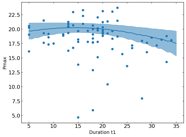
These plots show the relationship between a metric and a parameter. They show the predicted values of the metric on the y-axis as a function of the parameter on the x-axis while keeping all other parameters fixed at their status_quo value (or mean value if status_quo is unavailable).

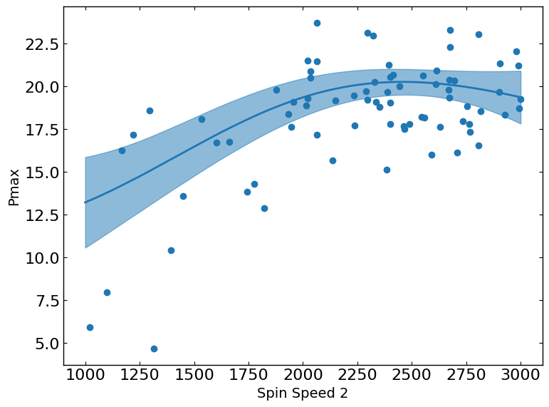
Spin_Speed_2 vs. Pmax

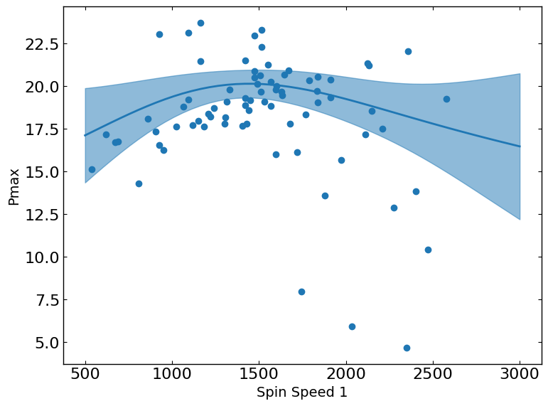
The slice plot provides a one-dimensional view of predicted outcomes for Pmax as a function of a single parameter, while keeping all other parameters fixed at their status_quo value (or mean value if status_quo is unavailable). This visualization helps in understanding the sensitivity and impact of changes in the selected parameter on the predicted metric outcomes.

Spin_Speed_1 vs. Pmax

The slice plot provides a one-dimensional view of predicted outcomes for Pmax as a function of a single parameter, while keeping all other parameters fixed at their status_quo value (or mean value if status_quo is unavailable). This visualization helps in understanding the sensitivity and impact of changes in the selected parameter on the predicted metric outcomes.

Contour Plots: Metric effects by parameter values

These plots show the relationship between a metric and two parameters. They show the predicted values of the metric (indicated by color) as a function of the two parameters on the x- and y-axes while keeping all other parameters fixed at their status_quo value (or mean value if status_quo is unavailable).

Spin_Speed_1, Spin_Speed_2 vs. Pmax

The contour plot visualizes the predicted outcomes for Pmax across a two-dimensional parameter space, with other parameters held fixed at their status_quo value (or mean value if status_quo is unavailable). This plot helps in identifying regions of optimal performance and understanding how changes in the selected parameters influence the predicted outcomes. Contour lines represent levels of constant predicted values, providing insights into the gradient and potential optima within the parameter space.

Diagnostic Analysis

Diagnostic Analyses provide information about the optimization process and the quality of the model fit. You can use this information to understand if the experimental design should be adjusted to improve optimization quality.

Cross Validation for Pmax

The cross-validation plot displays the model fit for each metric in the experiment. It employs a leave-one-out approach, where the model is trained on all data except one sample, which is used for validation. The plot shows the predicted outcome for the validation set on the y-axis against its actual value on the x-axis. Points that align closely with the dotted diagonal line indicate a strong model fit, signifying accurate predictions. Additionally, the plot includes 95% confidence intervals that provide insight into the noise in observations and the uncertainty in model predictions. A horizontal, flat line of predictions indicates that the model has not picked up on sufficient signal in the data, and instead is just predicting the mean.

from ax.utils.notebook.plotting import render# for plotting in notebook
from ax.plot.slice import plot_slice
from ax.plot.scatter import interact_fitted
from ax.adapter.cross_validation import cross_validate
from ax.plot.diagnostic import interact_cross_validation
from sklearn.metrics import r2_score

model = optimizer.ax_client._generation_strategy.adapter  # get the model from the ax client
cv_results = cross_validate(model)

# calculate the r2
observed, predicted = [], []
for i in range(len(cv_results)):
    observed.append(cv_results[i].observed.data.means[0])
    predicted.append(cv_results[i].predicted.means[0])
r2 = r2_score(observed, predicted)
print(f'R2 = {r2}')
render(interact_cross_validation(cv_results))

obj_type = 'Pmax' # objective type
p_idx = 0
for p_idx in range(len(optimizer.params)):
    x = ax.plot.slice.plot_slice(model=model,param_name= optimizer.params[p_idx].name, metric_name= obj_type).data['data'][1]['x']
    y = ax.plot.slice.plot_slice(model=model,param_name=optimizer.params[p_idx].name, metric_name= obj_type).data['data'][1]['y']
    x1 = ax.plot.slice.plot_slice(model=model,param_name= optimizer.params[p_idx].name, metric_name= obj_type).data['data'][0]['x']
    y1 = ax.plot.slice.plot_slice(model=model,param_name= optimizer.params[p_idx].name, metric_name= obj_type).data['data'][0]['y']
    # cut x1 and y1 to the same length as x and y
    x_low = x1[:len(x)]
    y_low = y1[:len(y)]
    x_high = x1[len(x):]
    y_high = y1[len(y):][::-1]

    plt.figure(figsize=(8,6))
    plt.plot(x,y)
    # shade the area between the two curves
    plt.fill_between(x, y_low, y_high, color='C0', alpha=0.5)
    # plt.fill_between(x, y, y_high, color='gray', alpha=0.5)
    plt.plot(data[optimizer.params[p_idx].name],data[obj_type],'C0o')
    plt.xlabel(optimizer.params[p_idx].display_name)
    plt.ylabel(obj_type)
    plt.tight_layout()
    plt.show()

R2 = 0.5015109633359836

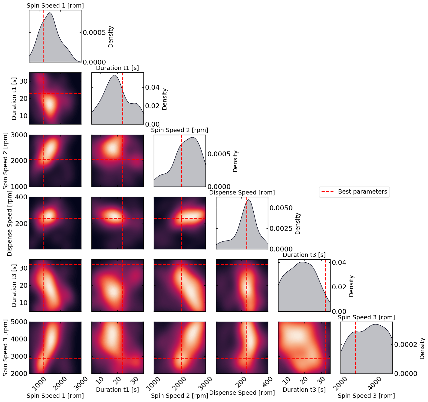
# Plot the density of the exploration of the parameters
# this gives a nice visualization of where the optimizer focused its exploration and may show some correlation between the parameters
plot_dens = True
if plot_dens:
    from optimpv.posterior.posterior import *
    params_orig_dict, best_parameters = {}, {}
    for p in optimizer.params:
        best_parameters[p.name] = p.value

    fig_dens, ax_dens = plot_density_exploration(params, optimizer = optimizer, best_parameters = best_parameters,  optimizer_type = 'ax')