OPV light-intensity dependant JV fits with SIMsalabim and Lazy posterior analysis (real data)

This notebook is a demonstration of how to fit light-intensity dependent JV curves with drift-diffusion models using the SIMsalabim package.

# Import necessary libraries
import warnings, os, sys, shutil
# remove warnings from the output
os.environ["PYTHONWARNINGS"] = "ignore"
warnings.filterwarnings(action='ignore', category=FutureWarning)
warnings.filterwarnings(action='ignore', category=UserWarning)
os.environ['PYTORCH_CUDA_ALLOC_CONF'] = 'expandable_segments:True'
import pandas as pd
import matplotlib.pyplot as plt
import numpy as np
from numpy.random import default_rng
import torch, copy, uuid
import pySIMsalabim as sim
from pySIMsalabim.experiments.JV_steady_state import *
import ax, logging
from ax.utils.notebook.plotting import init_notebook_plotting, render
init_notebook_plotting() # for Jupyter notebooks

try:
    from optimpv import *
    from optimpv.axBOtorch.axUtils import *
except Exception as e:
    sys.path.append('../') # add the path to the optimpv module
    from optimpv import *
    from optimpv.axBOtorch.axUtils import *

[INFO 12-08 08:22:00] ax.utils.notebook.plotting: Injecting Plotly library into cell. Do not overwrite or delete cell.
[INFO 12-08 08:22:00] ax.utils.notebook.plotting: Please see
    (https://ax.dev/tutorials/visualizations.html#Fix-for-plots-that-are-not-rendering)
    if visualizations are not rendering.

Get the experimental data

# Set the session path for the simulation and the input files
session_path = os.path.join(os.path.join(os.path.abspath('../'),'SIMsalabim','SimSS'))
input_path = os.path.join(os.path.join(os.path.join(os.path.abspath('../'),'Data','simsalabim_test_inputs','JVrealOPV')))
simulation_setup_filename = 'simulation_setup_PM6_L8BO.txt'
simulation_setup = os.path.join(session_path, simulation_setup_filename)

# path to the layer files defined in the simulation_setup file
l1 = 'ZnO.txt'
l2 = 'PM6_L8BO.txt'
l3 = 'BM_HTL.txt'
l1 = os.path.join(input_path, l1 )
l2 = os.path.join(input_path, l2 )
l3 = os.path.join(input_path, l3 )

# copy this files to session_path
force_copy = True
if not os.path.exists(session_path):
    os.makedirs(session_path)
for file in [l1,l2,l3,simulation_setup_filename]:
    file = os.path.join(input_path, os.path.basename(file))
    if force_copy or not os.path.exists(os.path.join(session_path, os.path.basename(file))):
        shutil.copyfile(file, os.path.join(session_path, os.path.basename(file)))
    else:
        print('File already exists: ',file)

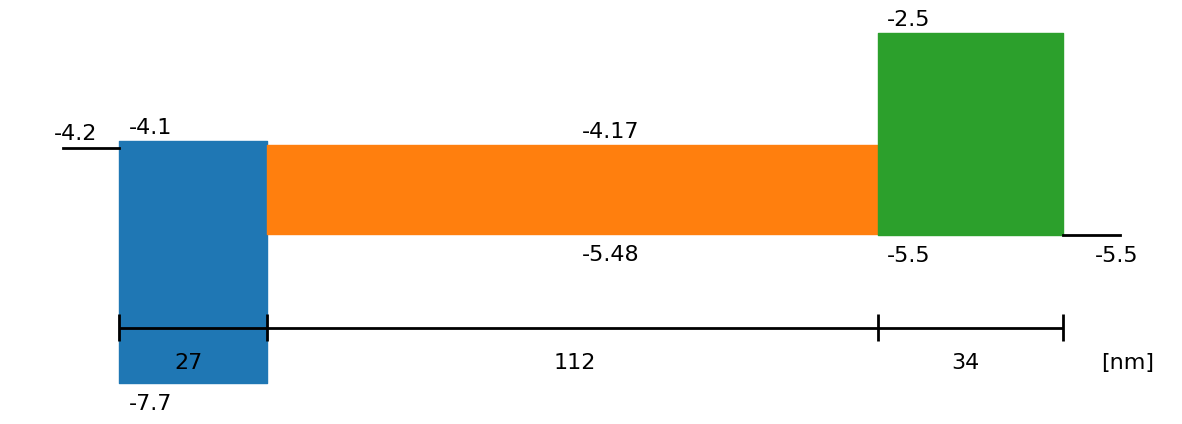
# Show the device structure
fig = sim.plot_band_diagram(simulation_setup, session_path)
dev_par, layers = sim.load_device_parameters(session_path, simulation_setup, run_mode = False)
SIMsalabim_params  = {}
for layer in layers:
    SIMsalabim_params[layer[1]] = sim.ReadParameterFile(os.path.join(session_path,layer[2]))
L_active_Layer = float(SIMsalabim_params['l2']['L'])

# Load the JV data
df = pd.read_csv(os.path.join(input_path, 'JV_PM6_L8BO.dat'), sep=' ')
X = df[['Vext','Gfrac']].values
y = df[['Jext']].values.reshape(-1)
Gfracs = pd.unique(df['Gfrac'])
X_1sun = df[['Vext','Gfrac']].values[df['Gfrac'] == 1.0]
y_1sun = df[['Jext']].values[df['Gfrac'] == 1.0].reshape(-1)

# get 1sun Jsc as it will help narrow down the range for Gehp
Jsc_1sun = np.interp(0.0, X_1sun[:,0], y_1sun)
minJ = np.min(y_1sun)
q = constants.value(u'elementary charge')
G_ehp_calc = abs(Jsc_1sun/(q*L_active_Layer))
G_ehp_max = abs(minJ/(q*L_active_Layer))
# get Voc
Voc_1sun = np.interp(0.0, y_1sun, X_1sun[:,0])

# Filter some data
Vmin = -0.1
Jmax = abs(Jsc_1sun)
idx = np.where((X[:,0] > Vmin) & (y < Jmax))
y = y[idx]
X = X[idx]

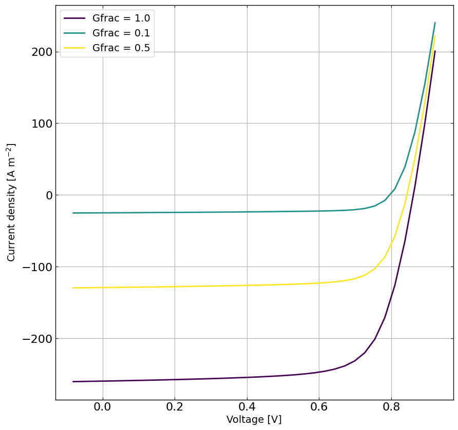
# plot the data for each Gfrac
plt.figure(figsize=(10,10))
viridis = plt.get_cmap('viridis', len(Gfracs))
for i, Gfrac in enumerate(Gfracs):
    plt.plot(X[X[:,1] == Gfrac][:,0], y[X[:,1] == Gfrac], '-', label = f'Gfrac = {Gfrac}', color = viridis(i))
plt.grid()
plt.xlabel('Voltage [V]')
plt.ylabel('Current density [A m$^{-2}$]')
plt.legend()

# calculate the sigma for the experimental data
std_phi = 0.05 # 5% error on light intensity
std_vol = 0.01 # 10 mV error on voltage

# reshape y such that each Gfrac is a column
y_reshaped = y.reshape((len(Gfracs), int(len(y)/len(Gfracs)))) # normalize to 10 A/m2
# print(y_reshaped)
# get dy/dGfrac
dJ_dphi = np.gradient(y_reshaped,Gfracs,axis=0,edge_order=2)
dJ_dV = np.gradient(y_reshaped,X[:,0][X[:,1]==Gfracs[0]],axis=1,edge_order=2)

phi_term = (std_phi * dJ_dphi)**2
vol_term = (std_vol * dJ_dV)**2
phi_term = phi_term.flatten()
vol_term = vol_term.flatten()
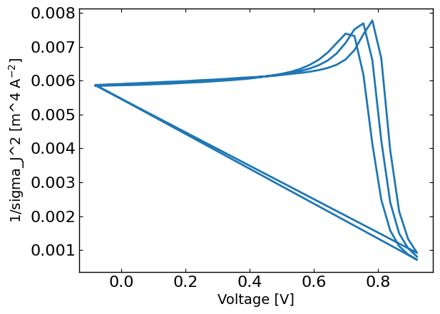
sigma_J = np.sqrt((std_phi*dJ_dphi)**2 + (std_vol*dJ_dV)**2)
# print((std_phi*dJ_dphi)**2, (std_vol*dJ_dV)**2)
# flatten sigma_J
sigma_J = sigma_J.flatten()  # convert to absolute error

plt.figure()
plt.plot(X[:,0],1/sigma_J**2)
plt.xlabel('Voltage [V]')
plt.ylabel('1/sigma_J^2 [m^4 A$^{-2}$]')
plt.show()
plt.show()

Define the parameters for the simulation

params = [] # list of parameters to be optimized

mun = FitParam(name = 'l2.mu_n', value = 7e-8, bounds = [5e-10,1e-6], log_scale = True, value_type = 'float', fscale = None, rescale = False, display_name=r'$\mu_n$', unit='m$^2$ V$^{-1}$s$^{-1}$', axis_type = 'log', force_log = True)
params.append(mun)

mup = FitParam(name = 'l2.mu_p', value = 5e-8, bounds = [5e-10,1e-6], log_scale = True, value_type = 'float', fscale = None, rescale = False, display_name=r'$\mu_p$', unit=r'm$^2$ V$^{-1}$s$^{-1}$', axis_type = 'log', force_log = True)
params.append(mup)

bulk_tr = FitParam(name = 'l2.N_t_bulk', value = 1e20, bounds = [1e17,1e22], log_scale = True, value_type = 'float', fscale = None, rescale = False,  display_name=r'$N_{T}$', unit=r'm$^{-3}$', axis_type = 'log', force_log = True)
params.append(bulk_tr)

preLangevin = FitParam(name = 'l2.preLangevin', value = 1e-2, bounds = [1e-3,1], log_scale = True, value_type = 'float', fscale = None, rescale = False, display_name=r'$\gamma_{pre}$', unit=r'', axis_type = 'log', force_log = True)
params.append(preLangevin)

R_series = FitParam(name = 'R_series', value = 1e-4, bounds = [1e-6,1e-2], log_scale = True, value_type = 'float', fscale = None, rescale = False,  display_name=r'$R_{series}$', unit=r'$\Omega$ m$^2$', axis_type = 'log', force_log = False)
params.append(R_series)

R_shunt = FitParam(name = 'R_shunt', value = 1e1, bounds = [1e-2,1e2], log_scale = True, value_type = 'float', fscale = None, rescale = False,  display_name=r'$R_{shunt}$', unit=r'$\Omega$ m$^2$', axis_type = 'log', force_log = False)
params.append(R_shunt)

G_ehp = FitParam(name = 'l2.G_ehp', value = G_ehp_calc, bounds = [G_ehp_calc*0.95,G_ehp_max*1.05], log_scale = False, value_type = 'float', fscale = None, rescale = False,  display_name=r'$G_{ehp}$', unit=r'm$^{-3}$ s$^{-1}$', axis_type = 'linear', force_log = False)
params.append(G_ehp)

# save the original parameters for later
params_orig = copy.deepcopy(params)

Run the optimization

# Define the Agent and the target metric/loss function
from optimpv.DDfits.JVAgent import JVAgent
metric = 'nrmse' # can be 'nrmse', 'mse', 'mae'
loss = 'linear' # can be 'linear', 'huber', 'soft_l1'
tracking_metrics = 'LLH' # can be 'nrmse', 'mse', 'mae', 'LLH'
tracking_loss = 'linear' # can be 'linear', 'huber', 'soft_l1'
tracking_weight = 1/sigma_J**2
tracking_X = X
tracking_y = y
tracking_exp_format = 'JV'
jv = JVAgent(params, X, y, session_path, simulation_setup, parallel = True, max_jobs = 3, metric = metric, loss = loss,tracking_metric = tracking_metrics, tracking_loss = tracking_loss,tracking_weight = tracking_weight,tracking_X=tracking_X, tracking_y=tracking_y, tracking_exp_format=tracking_exp_format)

import ray
import pandas as pd
from optimpv.axBOtorch.axBOtorchOptimizer import axBOtorchOptimizer
from optimpv.axBOtorch.axUtils import get_VMLC_default_model_kwargs_list

# Initialize Ray only once
if not ray.is_initialized():
    ray.init(ignore_reinit_error=True, num_cpus=180)

@ray.remote
def run_optimization_chain(chain_id, params, jv):
    """
    Ray remote version of a single optimization chain.
    """
    print(f"Starting optimization chain {chain_id}")

    num_free_params = len([p for p in params if p.type != "fixed"])

    optimizer = axBOtorchOptimizer(
        params=params,
        agents=jv,
        models=['SOBOL','BOTORCH_MODULAR'],
        n_batches=[2,100],
        batch_size=[10,2],
        ax_client=None,
        max_parallelism=-1,
        model_kwargs_list=get_VMLC_default_model_kwargs_list(
            num_free_params=num_free_params
        ),
        model_gen_kwargs_list=None,
        name=f'ax_opti_chain_{chain_id}',
        parallel=True,
        verbose_logging=False
    )

    optimizer.optimize_turbo()
    return optimizer.ax_client.summarize()


# -------------------------------
# Run all chains through Ray
# -------------------------------

n_chains = 10

# Launch all chains in parallel
futures = [
    run_optimization_chain.remote(i+1, params, jv)
    for i in range(n_chains)
]

# Collect results
results = ray.get(futures)

# Concatenate
data_main = pd.concat(results, ignore_index=True)

2025-12-08 08:22:05,242 INFO worker.py:2014 -- Started a local Ray instance. View the dashboard at http://127.0.0.1:8265 

(run_optimization_chain pid=1036977) Starting optimization chain 7

(run_optimization_chain pid=1036983) [WARNING 12-08 08:23:37] ax.api.client: Metric IMetric('JV_JV_LLH_linear') not found in optimization config, added as tracking metric.
(run_optimization_chain pid=1037020) [WARNING 12-08 08:23:46] ax.api.client: Metric IMetric('JV_JV_LLH_linear') not found in optimization config, added as tracking metric.
(run_optimization_chain pid=1036963) [WARNING 12-08 08:23:55] ax.api.client: Metric IMetric('JV_JV_LLH_linear') not found in optimization config, added as tracking metric.
(run_optimization_chain pid=1036973) [WARNING 12-08 08:24:12] ax.api.client: Metric IMetric('JV_JV_LLH_linear') not found in optimization config, added as tracking metric.
(run_optimization_chain pid=1036966) [WARNING 12-08 08:24:16] ax.api.client: Metric IMetric('JV_JV_LLH_linear') not found in optimization config, added as tracking metric.
(run_optimization_chain pid=1036974) [WARNING 12-08 08:24:22] ax.api.client: Metric IMetric('JV_JV_LLH_linear') not found in optimization config, added as tracking metric. [repeated 4x across cluster] (Ray deduplicates logs by default. Set RAY_DEDUP_LOGS=0 to disable log deduplication, or see https://docs.ray.io/en/master/ray-observability/user-guides/configure-logging.html#log-deduplication for more options.)

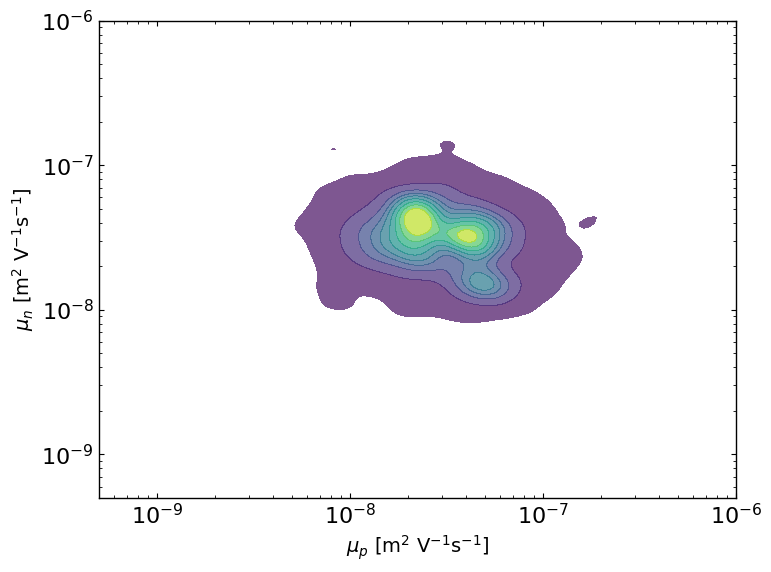
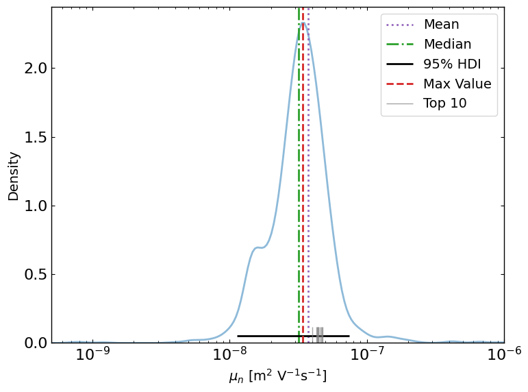
from optimpv.posterior.lazy_posterior import LazyPosterior
outcome_name = 'JV_JV_LLH_linear' #optimizer.all_tracking_metrics[0] #'LLH'
data_main = data_main[data_main['trial_index']>=20]
lazy_post = LazyPosterior(params, data_main, outcome_name)

ax = lazy_post.plot_lazyposterior_2D_kde('l2.mu_p','l2.mu_n',title=None)

ax2 = lazy_post.plot_lazyposterior_1D_kde('l2.mu_n',title=None,show_top_n=10)
ax2.legend()
plt.show()

# get the best parameters and update the params list in the optimizer and the agent
params_best = lazy_post.get_best_params()
params_median = lazy_post.get_top_n_metrics_params('median', num=10)
jv.params = params_best # update the params list in the agent with the best parameters

# print the best parameters
print('Best parameters:')
for p,po,pm in zip(params_best, params_orig, params_median):
    # print(p.name, 'fitted value:', p.value, 'original value:', po.value)
    if p.log_scale or p.force_log:
        print(f'{p.name} best fitted value: {p.value:.2e}, median value: {pm.value:.2e}')
    else:
        print(f'{p.name} best fitted value: {p.value}, median value: {pm.value}')

print('\nSimSS command line:')
print(jv.get_SIMsalabim_clean_cmd(jv.params)) # print the simss command line with the best parameters

Best parameters:
l2.mu_n best fitted value: 4.34e-08, median value: 4.42e-08
l2.mu_p best fitted value: 2.33e-08, median value: 2.30e-08
l2.N_t_bulk best fitted value: 3.03e+19, median value: 2.82e+19
l2.preLangevin best fitted value: 1.01e-03, median value: 1.01e-03
R_series best fitted value: 6.29e-05, median value: 6.32e-05
R_shunt best fitted value: 9.87e+01, median value: 9.75e+01
l2.G_ehp best fitted value: 1.4369711327011835e+28, median value: 1.4360270699531512e+28

SimSS command line:
./simss -l2.mu_n 4.340931155645187e-08 -l2.mu_p 2.3251607194508916e-08 -l2.N_t_bulk 3.0320564778787893e+19 -l2.preLangevin 0.0010098621778830952 -R_series 6.289623778437189e-05 -R_shunt 98.71660007212408 -l2.G_ehp 1.4369711327011835e+28

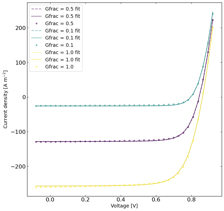
# rerun the simulation with the best parameters
yfit = jv.run(parameters={}) # run the simulation with the best parameters
jv.params = params_median
yfit_median = jv.run(parameters={}) # run the simulation with the best parameters
top_10_best_params_lst = lazy_post.get_top_n_best_params(10)
top_10_ys = []
for top_params in top_10_best_params_lst:
    jv.params = top_params
    y_top = jv.run(parameters={})
    top_10_ys.append(y_top)


viridis = plt.get_cmap('viridis', len(Gfracs))
plt.figure(figsize=(10,10))
linewidth = 2
for idx, Gfrac in enumerate(Gfracs[::-1]):
    for j, y_top in enumerate(top_10_ys):
        plt.plot(X[X[:,1]==Gfrac,0],y_top[X[:,1]==Gfrac],linestyle='-',color='k',alpha=0.05,linewidth=1,zorder=0)
    plt.plot(X[X[:,1]==Gfrac,0],yfit_median[X[:,1]==Gfrac],label='Gfrac = '+str(Gfrac)+' fit',linestyle='--',color=viridis(idx),alpha=0.5,linewidth=linewidth)
    plt.plot(X[X[:,1]==Gfrac,0],yfit[X[:,1]==Gfrac],label='Gfrac = '+str(Gfrac)+' fit',linestyle='-',color=viridis(idx),alpha=0.5,linewidth=linewidth)
    plt.plot(X[X[:,1]==Gfrac,0],y[X[:,1]==Gfrac],label='Gfrac = '+str(Gfrac),color=viridis(idx),alpha=0.5,linewidth=linewidth, marker='o', markersize=4,linestyle='None')

plt.xlabel('Voltage [V]')
plt.ylabel('Current density [A m$^{-2}$]')
plt.legend()
plt.show()

# Clean up the output files (comment out if you want to keep the output files)
sim.clean_all_output(session_path)
sim.delete_folders('tmp',session_path)
# uncomment the following lines to delete specific files
sim.clean_up_output('ZnO',session_path)
sim.clean_up_output('ActiveLayer',session_path)
sim.clean_up_output('BM_HTL',session_path)
sim.clean_up_output('simulation_setup_fakeOPV',session_path)