Bayesian Inference: Transient absorption spectroscopy fits with rate equation (fake data)

This notebook is a demonstration of how to fit transient absorption spectroscopy (TAS) with the following rate equations:

\[\frac{dn}{dt} = G - k_{trap} n - k_{direct} n^2\]

where \(n\) is the charge carrier density, \(G\) is the generation rate in m⁻³ s⁻¹, ktrap is the trapping rate in s⁻¹, and kdirect is the bimolecular/band-to-bad recombination rate in m³ s⁻¹.

The rate equation described here is the same as employed in the paper by Haffner‐Schirmer et al. 2017 to fit organic solar cell TAS data.

# Import necessary libraries
import warnings, os, sys, shutil
# remove warnings from the output
os.environ["PYTHONWARNINGS"] = "ignore"
warnings.filterwarnings(action='ignore', category=FutureWarning)
warnings.filterwarnings(action='ignore', category=UserWarning)
import pandas as pd
import matplotlib.pyplot as plt
import numpy as np
from numpy.random import default_rng
import torch, copy, uuid
import pySIMsalabim as sim
from pySIMsalabim.experiments.JV_steady_state import *
import ax, logging
from ax.utils.notebook.plotting import init_notebook_plotting, render
init_notebook_plotting() # for Jupyter notebooks

try:
    from optimpv import *
    from optimpv.RateEqfits.RateEqAgent import RateEqAgent
    from optimpv.RateEqfits.RateEqModel import *
    from optimpv.RateEqfits.Pumps import *
except Exception as e:
    sys.path.append('../') # add the path to the optimpv module
    from optimpv import *
    from optimpv.RateEqfits.RateEqAgent import RateEqAgent
    from optimpv.RateEqfits.RateEqModel import *
    from optimpv.RateEqfits.Pumps import *

[INFO 08-14 09:56:02] ax.utils.notebook.plotting: Injecting Plotly library into cell. Do not overwrite or delete cell.
[INFO 08-14 09:56:02] ax.utils.notebook.plotting: Please see
    (https://ax.dev/tutorials/visualizations.html#Fix-for-plots-that-are-not-rendering)
    if visualizations are not rendering.

Define the parameters for the simulation

# Define the parameters to be fitted
# Note: in general for log spaced value it is better to use the foce_log option when doing the Bayesian inference
params = []

k_direct = FitParam(name = 'k_direct', value = 5e-17, bounds = [1e-18,1e-16], log_scale = True, rescale = True, value_type = 'float', type='range', display_name=r'$k_{\text{direct}}$', unit='m$^{3}$ s$^{-1}$', axis_type = 'log',force_log=True)
params.append(k_direct)

k_trap = FitParam(name = 'k_trap', value = 1e6, bounds = [1e5,1e7], log_scale = True, rescale = True, value_type = 'float', type='range', display_name=r'$k_{\text{trap}}$', unit='s$^{-1}$', axis_type = 'log',force_log=True)
params.append(k_trap)

cross_section = FitParam(name = 'cross_section', value = 6e-21, bounds = [1e-21,1e-20], log_scale = True, rescale = True, value_type = 'float', type='range', display_name=r'$\sigma$', unit='m$^{2}$', axis_type = 'log',force_log=True)
params.append(cross_section)


# original values
params_orig = copy.deepcopy(params)
dum_dic = {}
for i in range(len(params)):
    if params[i].force_log:
        dum_dic[params[i].name] = np.log10(params[i].value)
    else:
        dum_dic[params[i].name] = params[i].value/params[i].fscale
   # we need this just to run the model to generate some fake data

Generate some fake data

Here we generate some fake data to fit. The data is generated using the same model as the one used for the fitting, so it is a good test of the fitting procedure.

# Define the necessary input parameters for the model
metric = 'mse'
loss = 'linear'
threshold = 10
exp_format = 'TAS'
P = 0.0039 # W
wavelegnth = 850e-9 # m
fpu = 1e5 # Hz
Area = 0.3*0.3*1e-4 # effective pump area in m^-2
penetration_depth = 1e-5*1e-2 # penetration depth in m
pulse_width = 0.2*(1/fpu) # width of the pump pulse in seconds
t0 = 0 # time offset of the pump pulse in seconds
background = 0 # background pump density in m^-3
# Calculate the average absorbed density in photons m^-3
flux, density = get_flux_density(P, wavelegnth, fpu, Area, penetration_depth)
pump_args = {'fpu': fpu , 'pulse_width': pulse_width, 't0': t0, 'P': density, 'background': background, }
fixed_model_args = {'L':100e-9}

t = np.linspace(0,1/fpu,1000)
t = t[:-1]

Gfracs = [0.1,0.5,1]
# concatenate the time and Gfracs
X = None
for Gfrac in Gfracs:
    if X is None:
        X = np.array([t,Gfrac*np.ones(len(t))]).T
    else:
        X = np.concatenate((X,np.array([t,Gfrac*np.ones(len(t))]).T),axis=0)

y_ = X # dummy data

RateEq_fake = RateEqAgent(params, [X], [y_], model = BT_model, pump_model = square_pump, pump_args = pump_args, fixed_model_args = fixed_model_args, metric = metric, loss = loss, threshold=threshold,minimize=True,exp_format=exp_format)

y = RateEq_fake.run(dum_dic,exp_format=exp_format)
noise = 1e-7
from numpy.random import default_rng
rng = default_rng()
y += rng.standard_normal(len(X))*noise

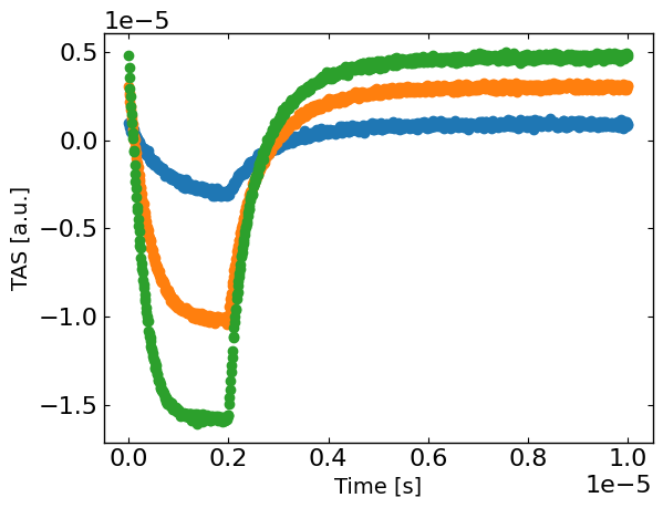
plt.figure()
for idx, Gfrac in enumerate(Gfracs):
    plt.plot(X[X[:,1]==Gfrac,0], y[X[:,1]==Gfrac],'o',label=str(Gfrac),)

plt.xlabel('Time [s]')
plt.ylabel(exp_format + ' [a.u.]')
plt.show()

Run the optimization

# Define the Agent and the target metric/loss function
metric = 'mse' # can be 'nrmse', 'mse', 'mae'
loss = 'linear' # can be 'linear', 'huber', 'soft_l1'

RateEq = RateEqAgent(params, [X], [y], model = BT_model, pump_model = square_pump, pump_args = pump_args, fixed_model_args = fixed_model_args, metric = metric, loss = loss, threshold=threshold,minimize=True,exp_format=exp_format)

MCMC Bayesian Inference for Parameter Fitting

We’ll use the emcee package to perform Markov Chain Monte Carlo sampling to find the posterior distribution of our model parameters.

from optimpv.BayesInfEmcee.EmceeOptimizer import EmceeOptimizer

# Define the Bayesian Inference object
optimizer = EmceeOptimizer(params = params, agents = RateEq, nwalkers=20, nsteps=1000, burn_in=100, progress=True, name='emcee_opti')

optimizer.optimize()

[INFO 08-14 09:56:03] optimpv.EmceeOptimizer: Running MCMC with 20 walkers for 1000 steps...

----------------------------------------------------

100%|██████████| 100/100 [00:18<00:00,  5.32it/s]
100%|██████████| 1000/1000 [03:31<00:00,  4.74it/s]
[INFO 08-14 09:59:55] optimpv.EmceeOptimizer: MCMC run complete.
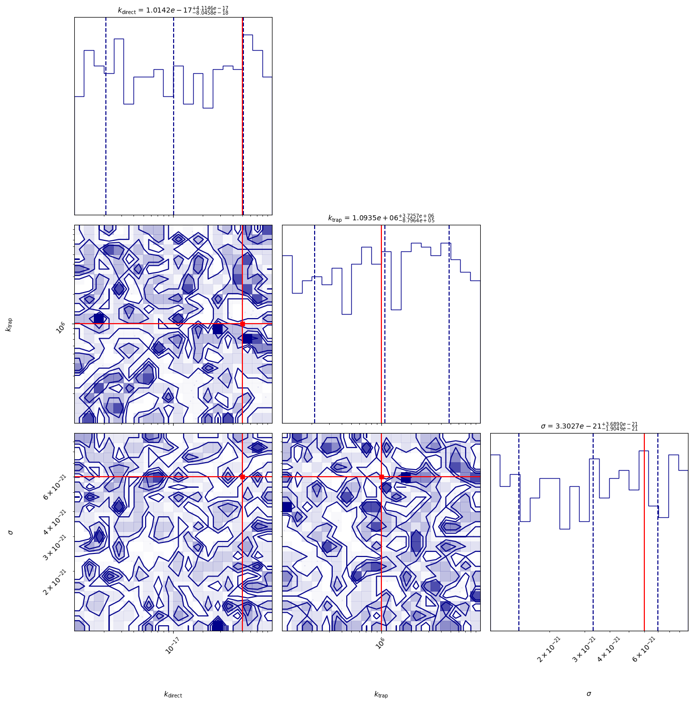
[INFO 08-14 09:59:55] optimpv.EmceeOptimizer: MCMC Results (Median & 16th/84th Percentiles)
[INFO 08-14 09:59:55] optimpv.EmceeOptimizer: $k_{\text{direct}}$ (k_direct): 1.013e-17 (+3.84e-17 / -8.03e-18)
[INFO 08-14 09:59:55] optimpv.EmceeOptimizer: $k_{\text{trap}}$ (k_trap): 1.447e+06 (+4.14e+06 / -1.19e+06)
[INFO 08-14 09:59:55] optimpv.EmceeOptimizer: $\sigma$ (cross_section): 3.204e-21 (+3.59e-21 / -1.74e-21)

----------------------------------------------------

{'k_direct': {'median': np.float64(1.0131945708970498e-17),
  '16th': np.float64(2.099120246850209e-18),
  '84th': np.float64(4.84967335777587e-17),
  'lower_err': np.float64(8.032825462120289e-18),
  'upper_err': np.float64(3.8364787868788205e-17)},
 'k_trap': {'median': np.float64(1447056.8108380437),
  '16th': np.float64(252589.75719231207),
  '84th': np.float64(5590677.227765576),
  'lower_err': np.float64(1194467.0536457316),
  'upper_err': np.float64(4143620.4169275323)},
 'cross_section': {'median': np.float64(3.204021307047606e-21),
  '16th': np.float64(1.4657468633269554e-21),
  '84th': np.float64(6.791503223287439e-21),
  'lower_err': np.float64(1.7382744437206506e-21),
  'upper_err': np.float64(3.5874819162398325e-21)}}

# corner plot
True_params = {p.name: p.value for p in params_orig} # Dictionary to hold true values for parameters
fig = optimizer.plot_corner(True_params=True_params) # Dictionary to hold true values for parameters

fig.set_size_inches(15, 15)

WARNING:root:Too few points to create valid contours
WARNING:root:Too few points to create valid contours

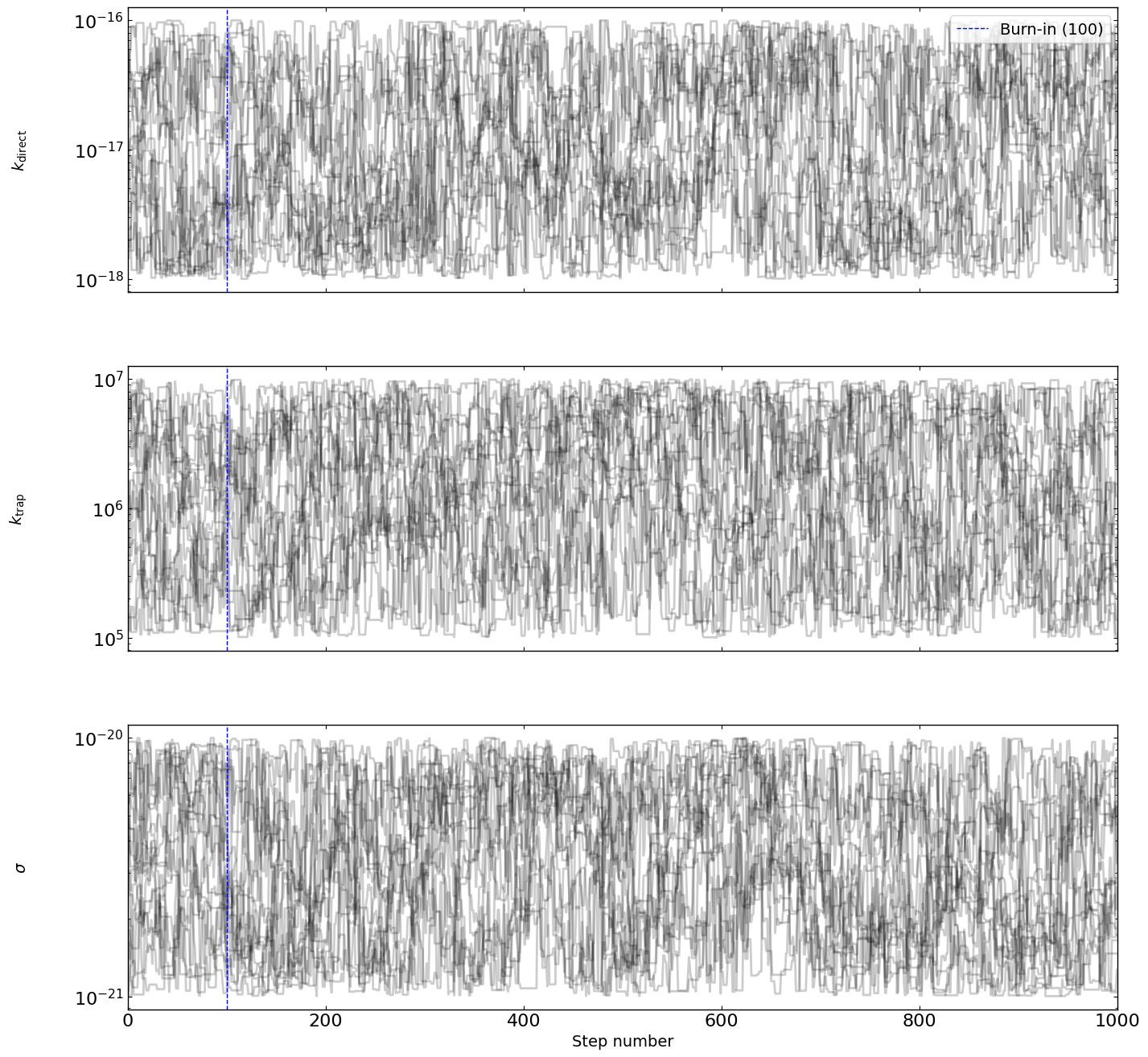
# optimizer.plot_trace()
fig = optimizer.plot_traces()
fig.set_size_inches(15, 15)

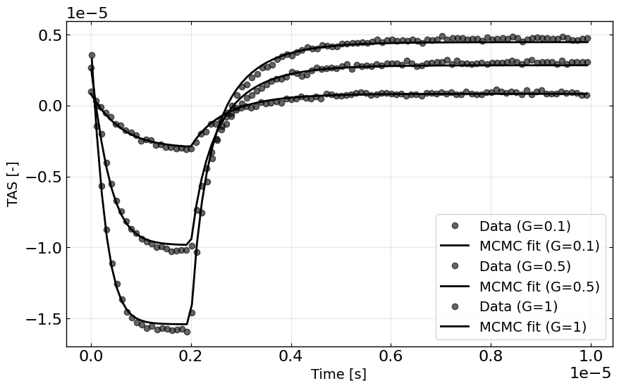
# Run simulation with best-fit parameters
best_fit_params = copy.deepcopy(optimizer.params)

# Create agent with best-fit parameters
best_agent = copy.deepcopy(RateEq)

best_fit_y = best_agent.run(parameters={},exp_format=exp_format)

# Plot the best-fit curves against data
plt.figure(figsize=(10, 6))
for Gfrac in Gfracs:

    # keep only every 10th point
    mask = np.zeros(len(X), dtype=bool)
    mask[::10] = True
    mask = np.logical_and(mask, X[:,1] == Gfrac)
    # mask = X[:,1] == Gfrac

    plt.plot(X[mask,0], y[mask], 'ko', alpha=0.6, label=f'Data (G={Gfrac})')
    plt.plot(X[mask,0], best_fit_y[mask], 'k-', label=f'MCMC fit (G={Gfrac})')

plt.xlabel('Time [s]')
plt.ylabel('TAS [-]')
plt.legend()
plt.grid(True, alpha=0.3)
plt.show()